Particle Filter Localization Project
Project Material
- Objectives
- Deliverables
- Deadlines & Submission
- Running the Code
- The Particle Filter Localization Description
- 1. Making a Map of the Environment
- 2. Initialializing Particles on the Map
- 3. Updating Particle Position/Orientation
- 4. Assigning Particle Weights Based on Sensor Measurements
- 5. Resampling
- 6. Updating Your Estimate of the Robot's Location
- 7. Optimization
- A View of the Goal
- A Personal Note
Objectives
Your goal in this project is to gain in-depth knowledge and experience with solving problem of robot localization using the particle filter algorithm. This problem set is designed to give you the opportunity to learn about probabilistic approaches within robotics and to continue to grow your skills in robot programming.
Learning Goals
- Continue gaining experience with ROS and robot programming
- Gain a hands-on learning experience with robot localization, and specifically the particle filter algorithm
- Learn about probabilistic approaches to solving robotics problems
Teaming & Logistics
You are expected to work with 1 other student for this project. Your project partner may be in a different lab section than you, however, both of you are expected to attend the same lab section for the next 2 weeks while you're working on this project. If you and your partner cannot attend the same lab section due to schedule conflicts, you will need to find a different partner. Your team will submit your code and writeup together (in 1 Github repo).
Selecting a partner: You can either choose your own partner, or you can can post in the #find-project-partner Slack channel that you're looking for a partner, and find someone else who's also looking for a partner.
Deliverables
Like last project, you'll set up your code repository using GitHub Classroom and submit your work on Gradescope (accessible via Canvas). The invite link to the GitHub Classroom can be found via the Canvas assignment for the Particle Filter Localization Project.
You'll want to put the particle_filter_project git repo within your ~/intro_robo_ws/src/ directory (where ROS2 packages should be located). Both partners will contribute to the same GitHub repo.
Implementation Plan
Please put your implementation plan within your README.md file. Your implementation plan should
contain the following:
- Names: The names of your team members
- Implementation and Testing:
A 1-2 sentence description of how your team plans to implement each of the following components of the particle filter localization as well as a 1-2 sentence description of how you will test each component to ensure that it is working correctly:
- How you will initialize your particle cloud (
initialize_particle_cloud)? - How you will update the position of the particles will be updated based on the movements of the robot
(
update_particles_with_motion_model)? - How you will compute the importance weights of each particle after receiving the robot's laser scan
data?(
update_particle_weights_with_measurement_model)? - How you will normalize the particles' importance weights (
normalize_particles) and resample the particles (resample_particles)? - How you will update the estimated pose of the robot (
update_estimated_robot_pose)? - How you will incorporate noise into your particle filter localization?
- How you will initialize your particle cloud (
- Timeline: A brief timeline sketching out when you would like to have accomplished each of the components listed above.
Writeup
Like last project, please modify the README.md file as your writeup for this project. Please add
pictures, Youtube videos, and/or embedded animated gifs to showcase and describe your work. Your writeup should:
- Objectives description (2-3 sentences): Describe the goal of this project.
- High-level description (1 paragraph): At a high-level, describe how you solved the problem of robot localization. What are the main components of your approach?
-
For each of the main steps of the particle filter localization, please provide the following:
- Code location (~1 sentence): Please describe where in your code you implemented this step of the particle filter localization.
- Functions/code description (1-3 sentences per function / portion of code): Describe the structure of your code. For the functions you wrote, describe what each of them does and how they contribute to this step of the particle filter localization.
- Initialization of particle cloud,
- Movement model,
- Measurement model,
- Resampling,
- Incorporation of noise,
- Updating estimated robot pose, and
- Optimization of parameters.
- gif or Embedded Video: You'll need to provide a gif or embedded video (e.g., embedded YouTube video) for each of your deliverables (initial and final). In both gifs/videos you need to show BOTH a view of your computer's screen showing the map and particles AND a view of the robot moving around in the maze.
- Initial deliverable gif/video: Show that the particles in your RViz window are moving as the robot moves around the maze. For this deliverable, we recommend using a very small number of particles (e.g., 10), so we can really see the particles moving as they should.
- Final deliverable gif/video: Showcase one of one of your most successful particle filter localization runs. In your gif/video, we should see the particles in your particle filter localization (visualized in RViz) converging on the actual location of the robot and a view of your robot in that same location in the maze.
- Challenges (1 paragraph): Describe the challenges you faced and how you overcame them.
- Future work (1 paragraph): If you had more time, how would you improve your particle filter localization?
- Takeaways (at least 2 bullet points with 2-3 sentences per bullet point): What are your key takeaways from this project that would help you/others in future robot programming assignments working in pairs? For each takeaway, provide a few sentences of elaboration.
- Use of genAI statement (1 bullet point per use of genAI): Describe how you used any generative AI tools or techniques in your project with one bullet point for each use of genAI. If you did not use any genAI tools, simply state, "I did not use any genAI tools in my work on this assignment." As a reminder, the genAI policy is listed on the syllabus page and details acceptable and unacceptable uses of genAI in this course.
Code
Following the GitHub Classroom invitation (located on the Canvas Particle Filter Project assignment), create a github repository for your team for this project, clone it within your ~/intro_robo_ws/src directory, re-build, and source the install/setup.bash file:
$ cd ~/intro_robo_ws
$ colcon build --symlink-install --packages-select particle_filter_project
$ source install/setup.bash
The starter code comes with the following files that enable you to run your code and visualize the map and particles:
particle_filter_project/particle_filter_launch.py
particle_filter_project/launch/visualize_particles_launch.py
particle_filter_project/rviz/visualize_particles_and_map.rviz
particle_filter_project/particle_filter_project/particle_filter.py
In addition to these files, you'll also create your own map of the maze, and store those files in a
maps folder in your particle_filter_project ROS package:
particle_filter_project/maps/maze_map.pgm
particle_filter_project/maps/maze_map.yaml
You will write your code within the particle_filter.py file we've provided.
Partner Contributions Survey
The final deliverable is ensuring that each team member completes this Partner Contributions Google Survey. The purpose of this survey is to accurately capture the contributions of each partner to your combined particle filter localization project deliverables.
Grading
The Partile Filter Project will be graded as follows:
- 5% Implementation Plan
-
20% Writeup
- 6% Objectives, High-level description, & gif/video
- 11% Main steps
- 3% Challenges, Future Work, Takeaways
- 20% Individual Contribution to Team
- 55% Code
- 47% Implementation of Main Components
- 4% Code Comments & Readability
- 3% Parameter Optimization/Experimentation
New to this project is the Individual Contribution grade. This will be assessed through your responses to the partner contributions survey. Your grade will reflect whether or not you made a significant contribution to both your team's (1) implementation (code, debugging) and (2) presentation (writeup, video, code comments).
Deadlines & Submission
- Thursday, October 16th 8:00pm - Implementation Plan
- Tuesday, October 21 8:00pm - Intermediate Deliverable: Particle Cloud Initalization & Movement
- Code: Complete the initalization of the particle cloud and motion model components of the project, i.e.,
initialize_particle_cloud()andupdate_particles_with_motion_model(). When we run your code, we should see the particles initalized within the boundaries of your map and when the robot moves, we expect to see your particles moving in the same way. - Writeup: Complete the warmup sections: objectives description, high-level description, and code location & functions/code description for (1) intialization of particle cloud and (2) movement model.
- gif / Embedded Video: Your gif/embedded video should show a small number (~10) of your particles being iniatlized in RViz and moving around in accordance with how the robot is moving. Your video should show both your RViz window and the robot.
- Code: Complete the initalization of the particle cloud and motion model components of the project, i.e.,
- Tuesday, October 28th 8:00pm - Code, Writeup, gif/video, Partner Contributions Survey
- In your final repository please keep all of the intermediate deliverable items (e.g., gif/embedded video), so you'll end up with multiple gifs/embedded videos in your final submission.
Running the Code
When you're ready to test your particle filter code on a Turtlebot4, connect to your robot and then run the following commands:
Terminal 1: visualize the map and particles - be sure that your map is named maze_map.yaml and is located in the ~/intro_robo_ws/src/particle_filter_project/maps directory.
$ ros2 launch particle_filter_project visualize_particles_launch.pyTerminal 2: teleoperate the robot using either the keyboard (recommended) or remote controller, if using the keyboard, be sure to specify the correct namespace based on your turtlebot4's number.
$ ros2 run teleop_twist_keyboard teleop_twist_keyboard --ros-args -r __ns:=/tb04Terminal 3: run the particle filter code (be sure to specify the correct namespace based on your turtlebot4's number)
$ ros2 launch particle_filter_project particle_filter_launch.py namespace:=/tb04The Particle Filter Localization
The goal of our particle filter localization (i.e., Monte Carlo localization) will be to help a robot answer the question of "where am I"? This problem assumes that the robot has a map of its environment, however, the robot either does not know or is unsure of its position and orientation within that environment.
To solve the localization problem, the particle filter localization approach (i.e., Monte Carlo Localization algorithm) makes many guesses (particles) for where it might think the robot could be, all over the map. Then, it compares what it's seeing (using its sensors) with what each guess (each particle) would see. Guesses that see similar things to the robot are more likely to be the true position of the robot. As the robot moves around in its environment, it should become clearer and clearer which guesses are the ones that are most likely to correspond to the actual robot's position. Please see the Class Meeting 04 page for more information about the MCL algorithm.
In more detail, the particle filter localization first initializes a set of particles in random locations and orientations within the map and then iterates over the following steps until the particles have converged to (hopefully) the position of the robot:
- Capture the movement of the robot from the robot's odometry
- Update the position and orientation of each of the particles based on the robot's movement
- Compare the laser scan of the robot with the hypothetical laser scan of each particle, assigning each particle a weight that corresponds to how similar the particle's hypothetical laser scan is to the robot's laser scan
- Resample with replacement a new set of particles probabilistically according to the particle weights
- Update your estimate of the robot's location
In the following sections, we'll walk through each of the main steps involved with programming your own particle filter localization algorithm.
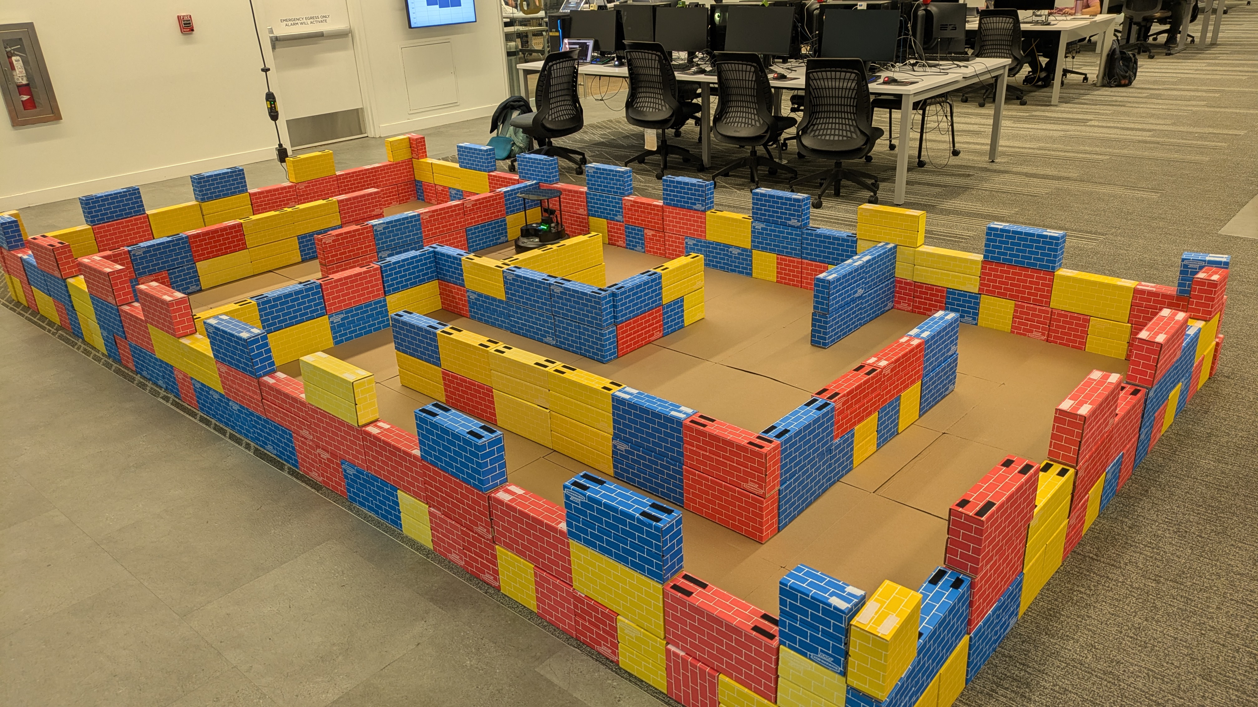
1. Making a Map of the Environment
Your first step with this project will involve recording a map of the maze (pictured below). Directions for recording the map can be found on the Lab C page. Please save your map in the particle_filter_project/maps directory under the name maze_map.
2. Initialializing Particles on the Map
Once you've created your map, you'll next want to initalize your particles. Ideally, you'll want your particles initiaized only within the light grey cells on the map (as opposed to the black obstacles/walls or the area outside the map), and randomly distributed across that area.
To initalize your particles within the map's boundaries, you'll need to work with the particle filter's map attribute, which is of type nav_msgs/OccupancyGrid. The map data list (data) uses row-major ordering and the map info contains useful information about the width, height, resolution, and more. You'll also want to locate the origin of the map to help you debug.
In order to visualize the particles on the map in RViz, you'll need to select the namespaced ROS2 topic in RViz (see gif below) that specifies the robot number you're working with (e.g., /tb10/particle_cloud when you're working with turtlebot4 number 10).

3. Updating Particle Position/Orientation Based on the Robot's Movement
Next, we need to ensure that when our robot moves around and turns (as you're teleoperating it), that the particles also move around and turn the exact same amount. You'll teleoperate the robot with either using either the keyboard or the remote controller. To keep track of the robot's movements, the starter code already computes the difference in the robot's xy position and orientation (yaw) in the robot_scan_received() function. If the robot moves "enough" based on the linear and angular movement thresholds, it will trigger one iteration of the particle filter localization algorithm.
Your job, is to use the precomputed difference in the robot's xy position and orientation (yaw) to update the particle positions, and also adding in some movement noise.
The gif below demonstrates an example of particles moving in accordance with the robot's movement. This example can also serve as a model for what the intermediate deliverable gif/video should look like (including both the RViz window and robot in the frame).

For example, we recommend you test out the movement of your particles by lowering your number of partcles to something like 4-10 particles and then observing their movement closesly to see if their movement matches that of the turtlebot.
4. Assigning Particle Weights Based on Sensor Measurements
This is a crticial component of the particle filter localization algorithm, where you assign a weight to each particle that represents how well the robot's sensor measurements match up with the particle's location on the map. As we went over in Class Meeting 05, you are welcome to use either a ray casting approach or a likelihood field approach.
One helper function we've provided you to assist with this section is compute_prob_zero_centered_gaussian(dist, sd). This function takes in a distance, which represents the difference between the LiDAR distance you receive from the robot and the distance you compute for your particle based on either the ray casting or likelihood field algorithm. With that input, the function outputs a probability value. For example, if your robot "sees" a distance of 2.0m at 90 degrees and your particle also "sees" a distance of 2.0m at 90 degrees, the distance value you'd feed into compute_prob_zero_centered_gaussian(dist, sd) would be 2.0 - 2.0 = 0, and you'd get a high probability output, since these values are closely aligned.
If you're implementing a likelihood field approach, you may find it useful to visualize your likelihood field as a helpful deubgging tool. Below is an example of how you might visualize your likelihood field.
import matplotlib.pyplot as plt

# reshape the likelihood field into a 2D array for visualization
likelihood_field_array = np.array(likelihood_field).reshape((self.map.info.height, self.map.info.width))

# plot the likelihood field
plt.imshow(likelihood_field_array, cmap="hot", interpolation="nearest")
plt.title("Likelihood Field")
plt.legend()
plt.colorbar()
plt.show()
Below is an example visualization of a likelihood field using the code above.

5. Resampling
After you've computed the particle weights, you'll now resample with replacement a new set of particles (from the prior set of particles) with a probability in proportion to the particle weights. You may find it helpful to use the numpy.random.choice() function for resampling.
Note that you MUST create a deep copy of each particle (not a shallow copy). Shallow copies represent pointers to the original particle and will not allow multiple copies of the same particle to hold different positions, orientations, and weights. To ensure that you're creating a deep copy of each particle, you'll need to create a new instance of the Particle class for each particle you want to copy.
6. Updating Your Estimate of the Robot's Location
Finally, you'll update the estimate of the robot's location based on the average position and orientation of ALL of the particles.
You will notice that your estimate will be very poor until your particles have begun to converge. This is ok and expected.
7. Optimization
Parameter and code optimization is a large component of student success in this project. Notably, this algorithm can be very computationally expensive, so it's important that you adjust your code and particle filter parameters to enable your particle filter localization code to run successfully.
Code Optimization: There are ways you can restructure your code to enable better performance, such as:
- Using numpy arrays instead of for loops
- Using a likelihood field measurement model approach instead of ray casting (however, we've seen both work in the past)
Parameter Optimization: There are many parameters you can adjust in your code to either (1) improve runtime performance and reduce lag or (2) improve the performance of the algorithm itself, some examples of paramters we encourage you to change and optimize include:
- The number of particles
- The number of laser scan measurements you incorporate into your measurement model
- The amount of noise you add to your particles' movement
A View of the Goal
The following example gifs show the progression of the particles over time. You can see that at the beginning, the particles are randomly distributed throughout the map. Over time, the particles converge on likely locations of the robot, based on its sensor measurements. And eventually, the particles converge on the true location of the robot.


And in this example of the Turtlebot3, you can see the particle filter side-by-side with the real robot in the maze.

A Personal Note
In many ways, I would not be a professor at UChicago and teaching this class had it not been for the particle filter that I programmed during my undergrad at Franklin W. Olin College of Engineering. My partner in crime, Keely, and I took a semester to learn about algorithms used in self-driving cars (under the guidance of Professor Lynn Stein) and implemented our own particle filter on a real robot within a maze that we constructed ourselves. It was this project that propelled me to get my PhD in Computer Science studying human-robot interaction, which then led me to UChicago. Below, I've included some photos of our project.


And here's the video of our particle filter working, where you can see the particles (blue) converging to the location of the robot (red).
Acknowledgments
The design of this course project was influenced by the particle filter project that Keely Haverstock and I completed in Fall 2012 at Olin College of Engineering as well as Paul Ruvolo and his Fall 2020 A Computational Introduction to Robotics course taught at Olin College of Engineering. The gifs and images providing examples of the particle filter are used with permission from former students Max Lederman, Emilia Lim, Shengjie Lin, Sam Nitkin, David Pan, Jett Yuen, and Connor Heron. Danny Lingen and Kendrick Xie also contributed in converting the Turtlebot3 & ROS1 version of this code to the Turtlebot4 & ROS2 version.