Project 1: 2D Particle Simulation with CUDA Optimizations

Due: Sunday, May 4th at 11:59pm

In this project, you will implement a 2D particle simulation using CUDA. Particles move based on simple physics (velocity, gravity), bounce off box walls, and interact via collisions with nearby particles. You will use various CUDA optimization techniques to accelerate performance and render frames to image files.

Using a GPU Resource

You are permitted to complete this assignment using either:

• The Midway3 cluster (via RCC), or

• The Peanut GPU cluster on the CS Linux servers

Please choose the environment that works best for you.

If you choose to work on the Peanut cluster, note that we you will need to profile your project on Midway3 until profiling works on the Peanut cluster. Please keep this in mind to ensure you leave enough time to profile on Midway3. Do not wait to start profiling until late in the assignment due date. We will not provide additional extensions in this case.

Creating Your Private Repository

To actually get your private repository, you will need this invitation URL:

• Project 1 invitation (Please check the Post “Project 1 is ready” Ed)

When you click on an invitation URL, you will have to complete the following steps:

1. You will need to select your CNetID from a list. This will allow us to know what student is associated with each GitHub account. This step is only done for the very first invitation you accept.

Note

If you are on the waiting list for this course you will not have a repository made for you until you are admitted into the course. I will post the starter code on Ed so you can work on the assignment until you are admitted into the course.

2. You must click “Accept this assignment” or your repository will not actually be created.

3. After accepting the assignment, Github will take a few minutes to create your repository. You should receive an email from Github when your repository is ready. Normally, it’s ready within seconds and you can just refresh the page.

4. You now need to clone your repository (i.e., download it to your machine).

   • Make sure you’ve set up SSH access on your GitHub account.

   • For each repository, you will need to get the SSH URL of the repository. To get this URL, log into GitHub and navigate to your project repository (take into account that you will have a different repository per project). Then, click on the green “Code” button, and make sure the “SSH” tab is selected. Your repository URL should look something like this: git@github.com:mpcs52072-spr25/proj1-GITHUB-USERNAME.git.

   • If you do not know how to use git clone to clone your repository then follow this guide that Github provides: Cloning a Repository

If you run into any issues, or need us to make any manual adjustments to your registration, please let us know via Ed Discussion.

Project 1: 2D Particle Simulation Overview

You will implement a 2D particle simulation using CUDA. Each particle represents a moving point with:

• A position: (x, y)

• A velocity: (vx, vy)

Particles move around the screen, bounce off the walls, and collide with nearby particles based on simple elastic collision rules.

The simulation runs for multiple time steps, and at each step you will:

1. Update particle positions using velocity and gravity

2. Detect and resolve collisions with nearby particles

3. Render the particle positions to a grayscale framebuffer

4. Save each frame as a .pgm image for visualization or animation

What Is a Particle?

Each particle is represented by a simple struct:

struct Particle {
    float x, y;   // position
    float vx, vy; // velocity
};

Note: You can choose to make this into a typedef, if you wish.

Framebuffer Rendering

The framebuffer is a 2D image (width × height) where each particle is drawn as a white pixel.

At each timestep:

• You clear the framebuffer

• You render all particle positions to it

• You save the image as a .pgm file

You will later use the provided script to convert these frames into an animated .gif.

Double Buffering (Required)

You must implement a double buffering system for updating particle positions and velocities in parallel.

Specifically:

• input: a buffer that holds the current state of all particles (positions + velocities)

• output: a second buffer where you write the updated particle states after each timestep

• After each frame, you swap these two buffers:

  • What was output becomes input for the next iteration

This pattern is required because:

• It prevents read/write conflicts (no thread reads and writes the same particle)

• It avoids race conditions when particles interact (e.g., collisions)

• It keeps your kernels clean, parallel-safe, and deterministic

Note

Swapping can be done by exchanging pointer references after each frame: Particle* temp = input; input = output; output = temp

Simulation Requirements

Your simulation must support:

• Multiple particles (hundreds to millions)

• Real-time updating of position using velocity and gravity

• Wall collisions

• Particle to particle collisions using elastic physics

• Saving a series of image frames representing the simulation

Task 1: Understanding the Program Usage

The following provides an explanation of the program usage for the simulation:

./simulation [-f <frames>] [-w <width>] [-h <height>] [-m <mode>] input_file output_dir

Flag	Description
input_file | Path to the particle input file (required).
-f <int>	Number of simulation frames to run (default: 100).
-w <int>	Width of the simulation grid in pixels (default: 800).
-h <int>	Height of the simulation grid in pixels (default: 600).
output_dir	Output directory for .pgm image frames (required).
-m <int>	Framebuffer memory mode: 0 = malloc, 1 = pinned, 2 = zero-copy. (default: 0)

Please note a few of these options will be explained in later sections of the specification.

Input File Format

The input file must be a text file structured as follows:

<number of particles>
x1 y1 vx1 vy1
x2 y2 vx2 vy2
...

Each line describes a particle’s:

• Initial position (x, y)

• Initial velocity (vx, vy)

Output

• The program will write one .pgm image per frame to the specified output directory. The name of each frame will have the following structure: input_file_N.pgm, where input_file is the base name of the input file provided on the command line, and N represents the frame this file represents.

• You can use the provided Python script (scripts/pgm_to_gif.py) to convert the frames into an animated .gif. In the same directory, it has an instructions document that explains the usage for the program.

As with the prior assignments no error-handling is necessary for command-line arguments.

Task 2: Implementing a Simulation Step

A single step in the particle simulation represents one unit of simulation time (e.g., one frame). In each step, your program must:

1. Update particle positions and velocities.

2. Detect and resolve collisions with nearby particles.

3. Render the particles into a framebuffer.

4. Swap simulation buffers for the next frame.

Physics Update

Each particle updates its position using basic kinematics:

vy += gravity;  // vertical acceleration (gravity = 9.8f)
x += vx;
y += vy;

If a particle hits a wall, it must bounce by inverting the appropriate velocity component:

if (x < 0 || x > width)  vx *= -1;
if (y < 0 || y > height) vy *= -1;

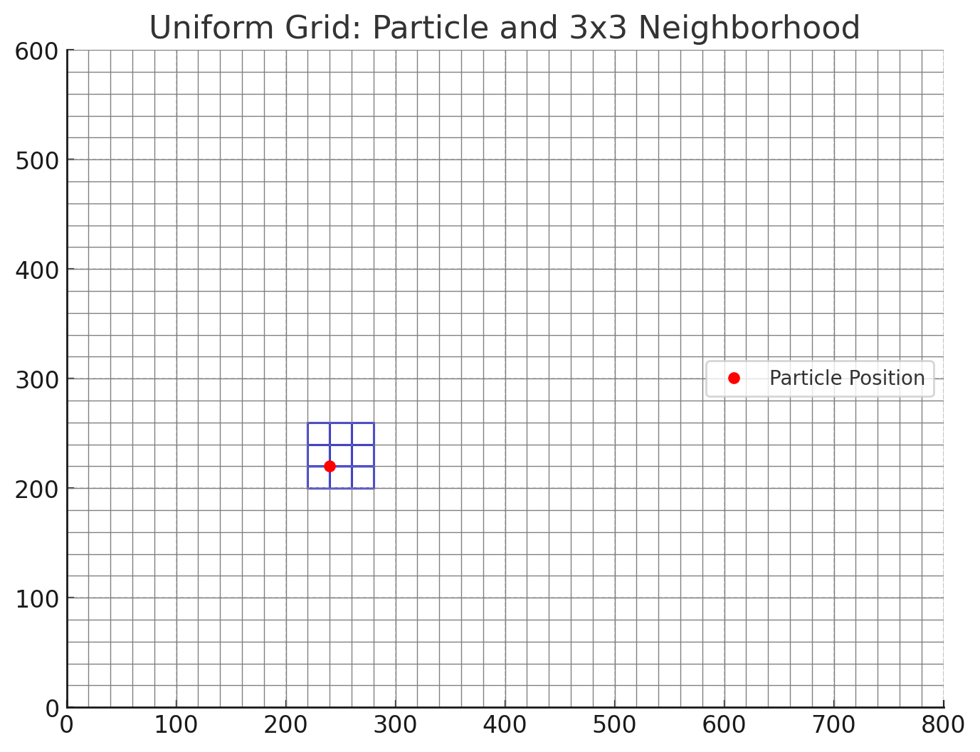
Uniform Grid: Collision Detection & Resolution

To reduce the number of pairwise particle comparisons, we use a uniform grid. This grid partitions the simulation space into fixed-size square cells. Each particle is assigned to a cell based on its position.

Why use it?

Instead of comparing every particle against every other particle (O(n²)), we:

• Assign each particle to a grid cell

• Only compare each particle to others in the same and neighboring cells (a 3x3 area)

• This reduces the cost of collision detection to O(n * k), where k is the average number of nearby particles

How it works:

Suppose each cell is CELL_SIZE × CELL_SIZE (e.g., 20×20 pixels), and your screen is 800 × 600.

Then your grid has:

GRID_COLS = width / CELL_SIZE  = 800 / 20 = 40
GRID_ROWS = height / CELL_SIZE = 600 / 20 = 30

Each particle belongs to a cell with:

int col = floor(x / CELL_SIZE);
int row = floor(y / CELL_SIZE);
int cell_id = row * GRID_COLS + col;

1. Preprocess the particles (CPU side):

   • Compute cell_id for each particle

   • Sort particles by cell_id (might want to use the C function qsort_r or qsort)

   • Record cell_start[cell_id] (i.e., the starting index in the sorted array) and cell_end[cell_id] (i.e., the last index for that cell) for each bucket. Note: This could also be done on the GPU side…

2. In the kernel:

   • For each particle, get its cell_id

   • Search for collisions in that cell and 8 neighbors (3x3 block)

   • Use cell_start and cell_end to restrict your loop to only relevant particles

The below diagram shows a visual representation of a uniform grid based on the assumptions above:

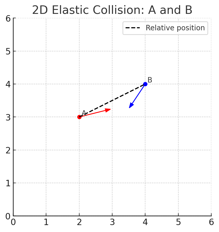
Elastic Collisions (2D, Equal Mass)

When two particles come close enough (within a defined radius), you apply an elastic collision to update their velocities.

Let’s say:

• Particle A has position A = (x1, y1) and velocity Va = (vx1, vy1)

• Particle B has position B = (x2, y2) and velocity Vb = (vx2, vy2)

A collision is detected using the following general idea:

Let:

• dx = x2 - x1

• dy = y2 - y1

• dvx = vx2 - vx1

• dvy = vy2 - vy1

Then:

float dot = dx * dvx + dy * dvy;
float dist2 = dx*dx + dy*dy;

if (dist2 > 0.0f && dist2 < radius² && dot < 0.0f) {
    float scale = dot / dist2;
    float cx = scale * dx;
    float cy = scale * dy;
    vx1 -= cx;
    vy1 -= cy;
}

This formula resolves a 2D collision assuming equal mass and perfect elasticity. A radius=4 is close enough for this project. The following provides a visual representation using the above assumptions:

Additional Guidance:

• Do not compare a particle with itself

• Avoid division by zero

• Only process updates if particles are moving toward each other (dot < 0)

Render the particles into a framebuffer

Each step of your simulation must produce a visual output — a grayscale image representing the current positions of all particles. This image is stored in a framebuffer, which acts as a virtual screen.

To ensure correct and conflict-free rendering, you must implement a double buffering strategy for your framebuffers:

• One buffer is the active framebuffer, where particle positions are rendered during the current frame.

• The other buffer is the render buffer, which holds the fully rendered image from the previous frame and is used to save the output as a .pgm file.

At each simulation step:

1. Clear the active framebuffer.

2. Render the current particle positions to the active framebuffer.

3. Save the render buffer to disk as a .pgm image.

4. Swap the two buffers: - The active framebuffer becomes the render buffer. - The previous render buffer becomes the new active framebuffer.

This strategy ensures:

• There are no read/write conflicts during rendering

• Each output image reflects a consistent snapshot of the simulation state

Over the course of the simulation, you will generate a sequence of images — one per frame — which can later be combined into an animation.

Framebuffer Characteristics

• Your framebuffer will represent a 2D grayscale image, one byte per pixel

• Each pixel should range in intensity from 0 (black) to 255 (white)

• Particles are rendered as individual white dots

You are expected to manage and allocate framebuffer memory appropriately, using one of three strategies explained below.

PGM Image Format

You must save the framebuffer as a .pgm image (Portable GrayMap). Use the “P5” binary format:

FILE* f = fopen("frame_0001.pgm", "wb");
fprintf(f, "P5\n%d %d\n255\n", width, height);
fwrite(framebuffer, 1, width * height, f);
fclose(f);

You should generate one image per frame of simulation. These can later be assembled into a .gif.

Framebuffer Memory Strategy

Your program must support three memory strategies for the framebuffers and benchmark their performance:

1. Regular memory: use malloc on the host and copy from device

2. Pinned memory: use cudaMallocHost and cudaMemcpy for faster transfers

3. Zero-copy: use cudaHostAllocMapped and allow the device to write directly to host memory

You must include benchmarks comparing transfer times and document your findings in your report.

Task 3: CUDA Optimization and Performance Expectations

You are expected to apply several CUDA optimization strategies that we’ve covered in class:

• Thread Coarsening

• Shared Memory with Tiling

• Parallel Scan

• Warp-Level Primitives

• Occupancy and Resource Utilization

Your implementation will be graded not only on correctness, but also on how effectively you apply these optimization techniques to achieve high performance and scalability.

It is your responsibility to determine where and how each optimization should be applied. We will not specify which techniques to use in specific parts of your code — discovering that is part of the challenge.

Note

You might be wondering: Do I need to implement all the optimizations specified above?

Yes, you do (with the exception of warp shufl functions are not required). However, one way to demonstrate your understanding is to implement multiple versions of the same kernel — for example, a global memory version and a shared memory version (as you did in HW3). You can then use your report to compare and contrast the tradeoffs of each approach:

This comparative analysis is encouraged and will be positively factored into grading, as it shows deeper reasoning and performance awareness.

Kernel Design Responsibility

Note that we are also not specifying which kernels to implement. This is up to you.

You must think carefully about:

• Which components make sense to run on the GPU

• Which components should remain on the host

Determining this breakdown is part of your design responsibility, and we will not provide guidance on this aspect.

Task 4: Project Report (Submit as report.md)

You are required to submit a brief written report alongside your code and output files. The purpose of the report is to reflect on the implementation and evaluation of the optimizations used in your particle simulation. Your report should be structured and include the following sections:

1. Kernel Analysis: Memory-Bound vs Compute-Bound

For each kernel you implemented, clearly identify whether the kernel is memory-bound or compute-bound. Use CUDA profiling tools such as Nsight Compute or nvprof to support your classification. Look for metrics like memory throughput, arithmetic instruction throughput, and achieved occupancy. Provide quantitative data (e.g., “memory throughput was 82%, arithmetic was 15%”) to support your reasoning.

Note: you could (not required) also estimate the ratio of arithmetic operations to memory operations (FLOPs per byte).

2. Optimization Strategies

For each of the following optimizations, describe:

• Where you implemented it (which kernel, what part of the computation)

• Why you applied the optimization at that location

• What performance impact you observed, if any

Optimizations to address:

• Thread Coarsening

• Shared Memory Tile Reuse

• Warp Shuffle Intrinsics

• Parallel Scan

• Parallel Scan (if implemented)

• Memory Coalescing

Include excerpts of your implementation and profiling results to support your discussion.

3. Occupancy and Launch Configuration

Discuss the occupancy of your key kernels:

• What was the achieved occupancy for each kernel?

• What values did you choose for your grid and block dimensions, and why?

• Did the number of particles or number of iterations affect the occupancy? Why or why not?

Use profiler outputs and metrics (e.g., waves per SM, active warps per SM, theoretical max occupancy) to justify your choices. Include graphs if helpful.

4. Framebuffer Memory Strategy Comparison

You must compare three framebuffer memory strategies:

• Regular host memory (malloc())

• Pinned host memory (cudaMallocHost())

• Zero-copy memory (cudaHostAllocMapped())

Run benchmarks varying:

• Number of particles (e.g., 100, 1,000, 10,000)

• Number of iterations (e.g., 1 frame vs 10 frames)

Report:

• Which memory strategy performed best, and under what conditions

• When the strategies produced similar performance

• Why you believe these patterns occurred

• How does the time per frame change over the course of multiple iterations?

• Is the performance steady or does it degrade or improve? Why might that be?

Support your answers with timing measurements and graphs.

Submission Format

• Submit your report as report.md or report.pdf

• Include all referenced plots and profiling output files

• Keep your report to around 2–3 pages if possible

Testing

Professor Samuels, will provide a few more test-cases towards of the end of fifth week. I first want you to test your own code and then will provide some additional tests later on to help you further debug.

Grading

Programming assignments will be graded according to a general rubric. Specifically, we will assign points for completeness, correctness, design, and style. (For more details on the categories, see our Assignment Rubric page.)

The exact weights for each category will vary from one assignment to another. For this assignment, the weights will be:

• Completeness and Correctness: 60%

• Design/Style: 15%

• Report Document: 25%

Submission

Before submitting, make sure you’ve added, committed, and pushed all your code to GitHub. You must submit your final work through Gradescope (linked from our Canvas site) in the “Project #1” assignment page via two ways,

1. Uploading from Github directly (recommended way): You can link your Github account to your Gradescope account and upload the correct repository based on the homework assignment. When you submit your homework, a pop window will appear. Click on “Github” and then “Connect to Github” to connect your Github account to Gradescope. Once you connect (you will only need to do this once), then you can select the repository you wish to upload and the branch (which should always be “main” or “master”) for this course.

2. Uploading via a Zip file: You can also upload a zip file of the homework directory. Please make sure you upload the entire directory and keep the initial structure the same as the starter code; otherwise, you run the risk of not passing the automated tests.

Note

For either option, you must upload the entire directory structure; otherwise, your automated test grade will not run correctly and you will be penalized if we have to manually run the tests. Going with the first option will do this automatically for you. You can always add additional directories and files (and even files/directories inside the stater directories) but the default directory/file structure must not change.

Depending on the assignment, once you submit your work, an “autograder” will run. This autograder should produce the same test results as when you run the code yourself; if it doesn’t, please let us know so we can look into it. A few other notes:

• You are allowed to make as many submissions as you want before the deadline.

• Please make sure you have read and understood our Late Submission Policy.

• Your completeness score is determined solely based on the automated tests, but we may adjust your score if you attempt to pass tests by rote (e.g., by writing code that hard-codes the expected output for each possible test input).

• Gradescope will report the test score it obtains when running your code. If there is a discrepancy between the score you get when running our grader script, and the score reported by Gradescope, please let us know so we can take a look at it.