Project #1: Schelling’s Model of Housing Segregation¶

Due: Saturday, July 27, 11:59pm CDT

The goal of this project is to have you apply the optimizations we discussed in lecture up to this point and apply it to running a simulation on a GPU.

Peanut Cluster and GPU Partitions¶

If you are not familiar with submitting jobs to a cluster (i.e., the Peanut cluster) please make sure to watch the following video and read over the SLURM documentation provided by our tech-staff before beginning the assignment:

We will grade all assignments using the Peanut cluster’s GPUs and all programming assignments must work correctly on one of these machines. If you have a NVIDIA GPU installed on your local machine then you can work; however, your program must still work on one of the cluster’s GPU nodes, no exceptions.

You have the option batching your programs to the following cluster nodes

PARTITION AVAIL TIMELIMIT NODES STATE NODELIST
gpu-all up 4:00:00 2 idle gpu[2-3]
titan up 4:00:00 1 idle gpu3
pascal up 4:00:00 1 idle gpu2
quadro up 4:00:00 1 idle gpu1

Please be cautious of using titan since it’s been known to have stalling problems so we advise not using it until it’s been reliably fixed.

Creating Your Private Repository¶

To actually get your private repository, you will need this invitation URL:

Project 1 invitation (Please check the Post “Project 1 is ready” Ed)

When you click on an invitation URL, you will have to complete the following steps:

You will need to select your CNetID from a list. This will allow us to know what student is associated with each GitHub account. This step is only done for the very first invitation you accept.

Note

If you are on the waiting list for this course you will not have a repository made for you until you are admitted into the course. I will post the starter code on Ed so you can work on the assignment until you are admitted into the course.

You must click “Accept this assignment” or your repository will not actually be created.
After accepting the assignment, Github will take a few minutes to create your repository. You should receive an email from Github when your repository is ready. Normally, it’s ready within seconds and you can just refresh the page.
You now need to clone your repository (i.e., download it to your machine).
- Make sure you’ve set up SSH access on your GitHub account.
- For each repository, you will need to get the SSH URL of the repository. To get this URL, log into GitHub and navigate to your project repository (take into account that you will have a different repository per project). Then, click on the green “Code” button, and make sure the “SSH” tab is selected. Your repository URL should look something like this: git@github.com:mpcs52072-sum24/proj1-GITHUB-USERNAME.git.
- If you do not know how to use git clone to clone your repository then follow this guide that Github provides: Cloning a Repository

If you run into any issues, or need us to make any manual adjustments to your registration, please let us know via Ed Discussion.

Introduction¶

The New York Times had an interesting toolfor viewing the distribution of racial and ethnic groups in cities and states around the country. If you look at the map for the Greater Chicago area, you will see that many areas are heavily segregated, but that some, such as the suburb of Glendale Heights, are not. The forces that led to this arrangement of people are complex and it is unlikely that any simple model can truly answer the questions of how segregation arises and why it persists. Keeping that in mind, one can still ask simple questions that may shed some light on the situation. In his 1978 book Micromotive and Macrobehavior, Thomas Schelling considered the following question: is it possible that a group of individuals would prefer to live in integrated neighborhoods and yet, as the result of their collective choices end up in segregated neighborhoods?

Schelling examined this question using a very simple model: A city has two kinds of people, Cubs fans and White Sox fans, for example, and each person in the city requires a certain number of their neighbors to be like them to feel comfortable in their location. Schelling used this model to study the patterns that emerge if, over time, people who are unsatisfied with their initial locations or become unsatisfied over time relocate to new locations that satisfy their criteria. What happens depends on the ratio of the two populations and on the satisfaction criteria used by the individuals, but segregation is a frequent outcome.

Schelling’s model of housing segregation has led to myriad follow-up work examining different facets of the model’s outcomes in different circumstances, as well as applying the model to longitudinal datasets of urban environments. Data about Chicago features in a number of these analyses.

Task #0: Understanding Our Model¶

Your task in this project will be to implement a variant of Schelling’s model on a GPU. Before you can do so, we need to specify the details of the abstract model we will be using and then describe the concrete data structures we will be using to implement the model.

For the model, we need to specify, the:

shape and composition of a city,
boundaries of a home’s neighborhood,
definition for a similarity score,
definition for satisfaction,
rule for relocating homeowners,
composition of a relocation wave in the simulation,
composition of a step in the simulation, and
stopping conditions for the simulation.

Cities¶

A city is modelled as an $N \times N$ grid (where the value of $N$ can be different for each city). Each grid location (or cell) represents a home, which can be for sale, occupied by a maroon homeowner, or occupied by a blue homeowner. You may assume that a city has at least one home for sale and homes that are for sale are not occupied.

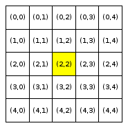
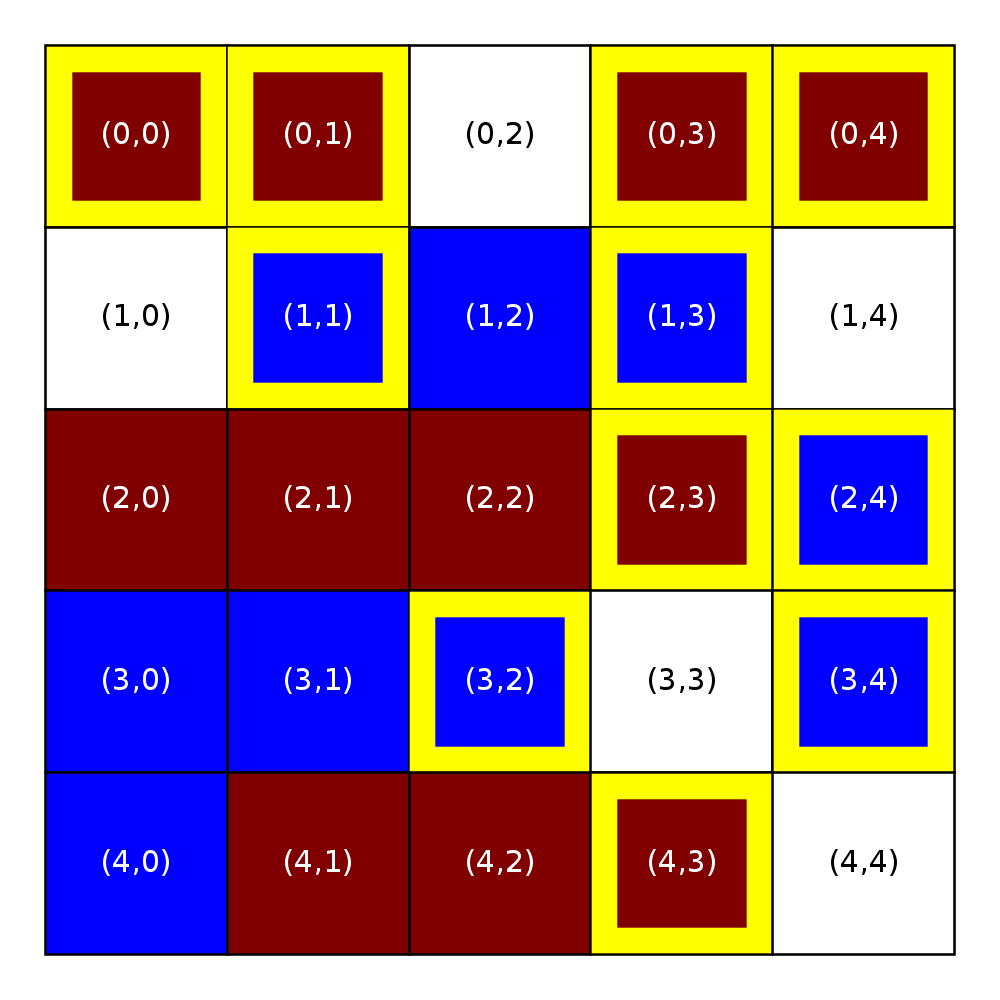
Here is a sample city that we will use throughout this write-up:

Sample City

In this and in nearly all subsequent city depictions, a white cell indicates a home that is for sale (i.e., unoccupied home), a maroon (dark red) cell indicates that a home is occupied by a maroon homeowner, and a blue cell indicates a home that is occupied by a blue homeowner. This figure also includes the location (in parentheses) of each home (cell) to help orient you in the city.

Neighborhood¶

The neighborhood of a home will be defined by a parameter R (this radius value will be an input to the model, so the value of R may vary from one simulation to another). The R-neighborhood of the home at Location $(i,j)$ contains all Locations $(k,l)$ such that:

$0 \le k \lt N$ and $i-R \le k \le i+R$
$0 \le l \lt N$ and $j-R \le l \le j+R$

Note that the Location $(i,j)$ itself is considered part of its own neighborhood. Thus, every homeowner will have at least one neighbor (themselves).

We will refer to a neighborhood with parameter R=x as an “R-x neighborhood”. The following figure shows the neighborhoods around Locations (2,2) and (3,0) for different values of R. Cells colored yellow are included in the specified neighborhood.

Neighborhood around (2,2)		Neighborhood around (3,0)
R = 0	R = 1	R = 1	R = 2

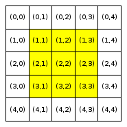
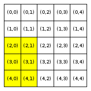
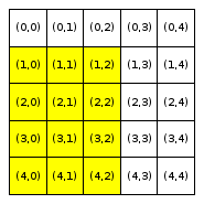
Notice that Location (3,0), which is closer to the boundaries of the city, has fewer neighboring homes for the same value of R than Location (2,2), which is the middle of the city. We use the term boundary neighborhood to refer to a neighborhood that is near the boundary of the city and thus does not have a full set of neighbors.

Color of homeowner¶

We define two groups of homeowners: maroon homeowners and blue homeowners. Homeowners of a particular group prefer to live in a neighborhood where at least some given fraction of their neighbors are from the same group as them. That is, maroon homeowners prefer that at least some minimum fraction of their neighbors are also maroon, while blue homeowners prefer that at least some minimum fraction of their neighbors are also blue.

Throughout the assignment, maroon homeowners will be indicated with an M while blue homeowners will be indicated with a B.

Satisfaction¶

For each homeowner, we are going to compute two scores to determine whether they are satisfied:

We define the similarity score to be S/H where S is the number of homes in the neighborhood with occupants of the same color as the homeowner and H is the number of occupied homes in the neighborhood.
We define the occupancy score to be H/T where H is as defined previously, and T is the total number of locations (occupied and unoccupied) in the neighborhood.

Since a homeowner is included in their own neighborhood, S, T, and H will each be at least one. A homeowner is satisfied with their location if their similarity score is greater than or equal to a specified similarity threshold and their occupancy score is greater than or equal to a specified occupancy threshold. This models takes into consideration homeowners may want to live in neighborhoods with similar homeowners, but may also want to avoid neighborhoods with a lot of unoccupied homes (even if the occupied homes have similar homeowners, the empty homes could be a sign of trouble in the neighborhood).

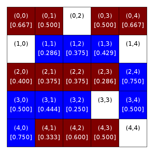
The figures below illustrate this concept using a city with R-1 neighborhoods. They show homeowners and their similarity scores (on the left figure) and their occupancy scores (on the right figure). White cells depict unoccupied homes/locations. Cells that are maroon (dark red) contain maroon homeowners. Cells that are blue contain blue homeowners. Each grid cell contains its location (in parentheses) and, for occupied homes, the homeowner’s R-1 similarity or occupancy score (in square brackets). We rounded the scores in the figures to three digits merely for clarity. Do not round them in your computation.

Similarity scores	Occupancy scores
R=1	R=1

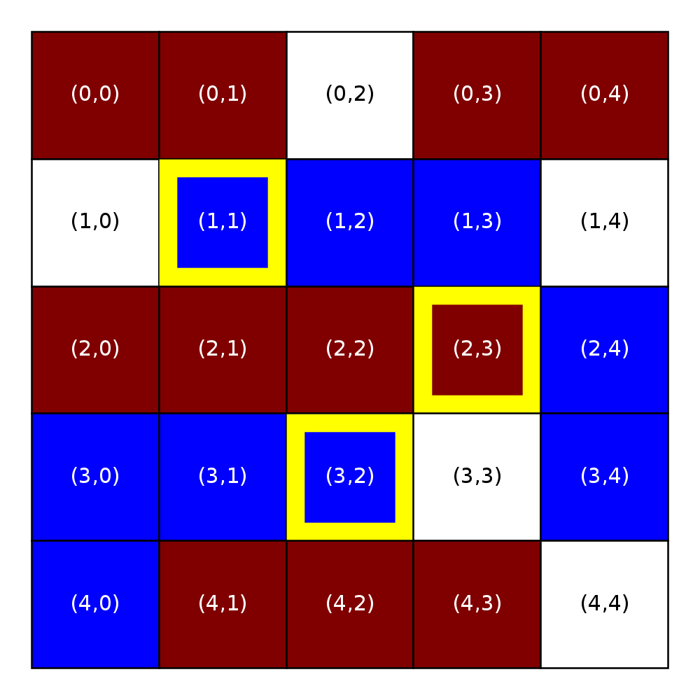
We will then determine which homeowners are satisfied, and which are not, based on the similarity and occupancy thresholds. For simplicity, let’s start by looking at what happens when the similarity threshold is 0.33 but the occupancy threshold is zero (i.e., when the occupancy score has no effect on whether a homeowner is satisfied or not).

Throughout this assignment, we indicate unsatisfied homeowners with a yellow border.

Similarity threshold = 0.33
Occupancy threshold = 0.00
R=1

The next two figures will illustrate the impact of the similarity threshold on satisfaction. The figure on the left is the same as the one above (similarity threshold of 0.33 and an occupancy threshold of 0.00). The figure on the right shows what happens when we raise the similarity threshold to 0.40. Notice how there are now more unsatisfied homeowners. If you look back at the figure with the similarity threshold, you’ll see that the unsatisfied homeowners that appear in the right figure but not in the left figure are those with a similarity score between 0.33 and 0.40

Similarity threshold = 0.33	Similarity threshold = 0.40
Occupancy threshold = 0.00	Occupancy threshold = 0.00
R=1	R=1

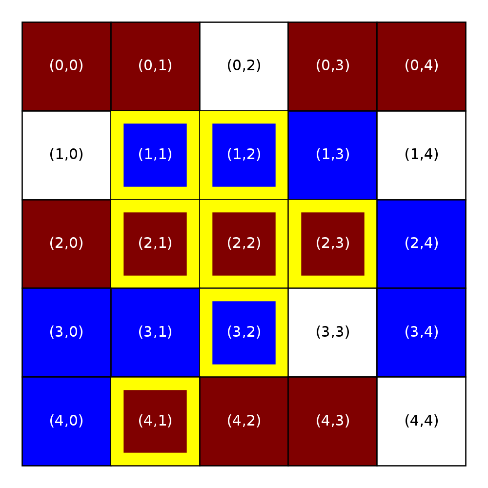
Notice how the homeowner at (2,0), with similarity score 0.400, is still satisfied in the right figure, because a homeowner will be satisfied if their similarity score is greater than or equal to the similarity threshold.

Next, we will further illustrate the impact of the threshold on satisfaction through two examples in which the occupancy threshold is greater than zero.

Similarity threshold = 0.33	Similarity threshold = 0.33
Occupancy threshold = 0.70	Occupancy threshold = 0.80
R=1	R=1

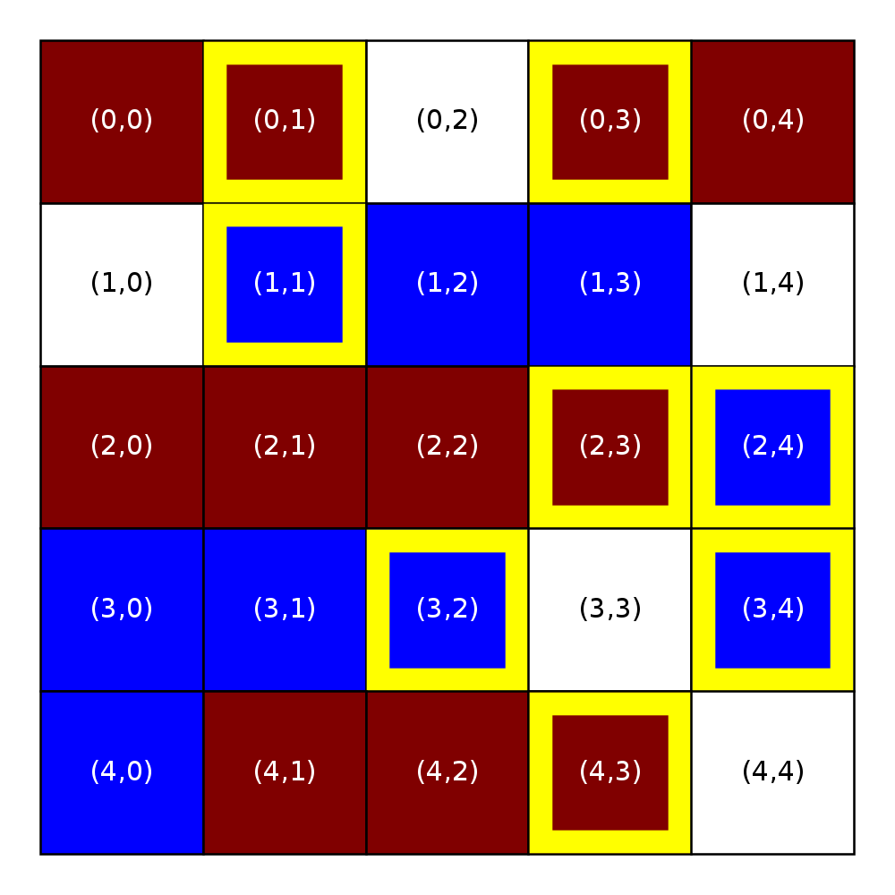
Notice how, relative to the figure with a similarity threshold of 0.33 and an occupancy threshold of 0.00, the left figure has more unsatisfied homeowners (those with an occupancy score below 0.70). Raising the occupancy threshold to 0.80 results in a few more unsatisfied homeowners, such as the one in (0,4): That homeowner’s similarity score (0.667) is above the similarity threshold, but their occupancy score (0.75) is not above the occupancy threshold.

Relocation rule¶

Homeowners who are unsatisfied will try to move as far away as possible from their current neighborhood to see if they will become satisfied in a far way location. You will calculate the distance between ($r_{1}$, $c_{1}$) and ($r_{2}$, $c_{2}$) using Manhattan distance:

\[Distance = |r_{2} - r_{1}| + |c_{2} - c_{1}|\]

For example, the distance between (2,2) and (4,2) on the grid is $2$. The distance between (2,3) and (1,1) is $3$. Note that if a homeowner’s current home is already satisfactory, then that is where they wish to live because the home is satisfactory.

However, sometimes homeowners will have multiple homes to choose from at the same (far) distance. In these cases, homeowners assume that a home that has been vacant for a while might suffer from issues, the homeowner will prefer homes that have been unoccupied for the shortest amount of time. If multiple homes have the same shortest amount of time then choose the empty home that comes first in row-major order.

To state these preferences more precisely: given multiple (unoccupied) homes, an unsatisfied homeowner will choose the farthest home (the home with the maximum distance from the homeowner’s current location). In the case of ties, the homeowner will choose the home that has been on the market shortest from among those remaining. the homeowner will not relocate if there are no available empty locations.

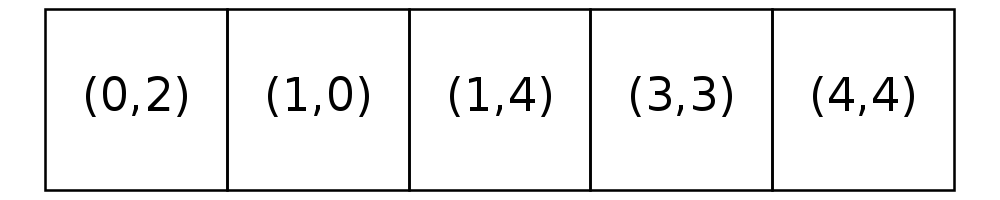
Here is an example relocation of the unsatisfied homeowner at Location (1,1) to Location (0,2). On the left, we show a city with R-1 neighborhoods in which the similarity threshold is 0.44 and the occupancy threshold is 0.5. Below the grid, we also include a depiction of the locations that are open in the neighborhood.

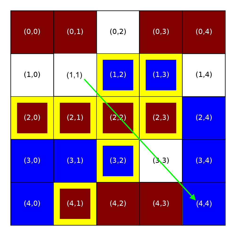
Before relocation	After relocation

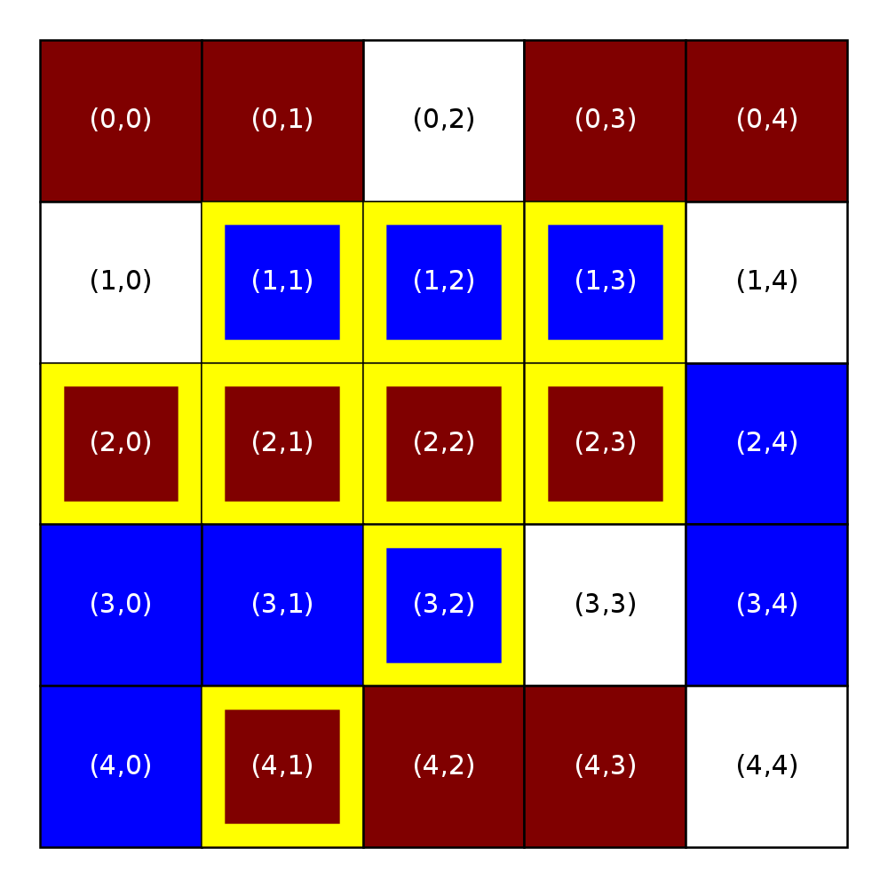
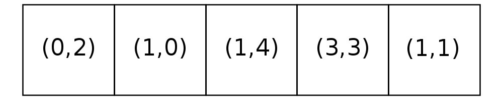
The blue homeowner in Location (1,1) is unsatisfied with their location. They consider all five open locations and find the following:

Location	Distance
Location (0,2)	2
Location (1,0)	1
Location (1,4)	3
Location (3,3)	4
Location (4,4)	6

the homeowner chooses among these four locations by choosing the one that is farthest, which is (4,4) in this case. Had more than one of these locations been equally close, the homeowner would have moved to the location that had been on the market the shortest.

The frame on the right shows the state of the empty list after this relocation. Notice that location (4,4) has been removed from the list of open locations and location (1,1) has been added to the end of the list. The blue owner is now at location (4,4). With this move, other neighboring homewoners may become unsatisfied, even the blue neighbor may not be satisfied with this move; however, we will not recalculate satisfaction until the next simulation step.

Simulation Step¶

A step in the simulation consists of the following:

Makes a pass over the city to calculate the homeowners who are satisfied and unsatisfied as described above.
Relocate each unsatisfied homeowner (if possible).
Repeat #1 if one of the stopping conditions (described below) have not been met.

Stopping conditions¶

We will simulate steps until we have met one of the following criteria:

Executed a specified maximum number of simulation steps.
Executed a step that had zero relocations.
After Step #1 (in Simulation Step section) the percentage of satisfied homeowners is above a specified maximum satisfaction threshold.

Program Structure & Files¶

Inside proj1/schelling.cu, you will implement our model described above. You will read in the city information from a file. The file will have the following format

The first line is a single integer representing the neighbor radius R.
The second line is a single floating point number representing similarity threshold. The value will always be between [0.0,1.0].
The third line is a single floating point number representing occupancy threshold. The value will always be between [0.0,1.0].
The fourth line is a single integer that represents the maximum number of simulation steps.
The fifth line is a single integer that represent the maximum satisfaction threshold. The value will always be between [0.0,1.0].
The sixth line is a single integer representing $N$ dimension of the city.
All remaining lines represent the rows and columns of the city. Each line represent a row of the city. Each column is a single capital character that is either: a B which represents a blue homeowner, M which represents a maroon homeowner, and E that represents an empty home (i.e., unoccupied home). Each character is separated by a single whitespace.

Here’s a file in data/sample-city.txt that represents the sample city described in the above sections.

1
0.33
0.70
20
0.78
5
M M E M M
E B B B E
M M M M B
B B B E B
B M M M E

The usage for this program takes in a single file that represents the city configuration and simulation parameters.

Usage: schelling configuration_file
   configuration_file - the file containing the city layout and simulation parameters

You will notice that proj1/schelling.cu is empty. You will be implementing everything from scratch for this assignment.

Program Output¶

The output of the program is the total number of fully completed simulation steps. A simulation step is fully completed if it’s able to complete all three steps specified in section Simulation Step. As a reminder, a step can be partially completed if the percentage of satisfied homeowners is above the maximum satisfaction threshold.

Task #1: GPU Implementation¶

For this assignment, you will take full control over how to implement this model on the GPU. You must take into consideration all the optimizations we discussed throughout modules 1-4 when designing and implementing your solution. How you will be graded will be based off correctness but also on whether you choose appropriate optimizations. Please do not ask on Ed for us to review your design or implementation choices. This is what we are grading you on! You are not required to write a sequential version of this model. You only need to implement a GPU version. It might be the case that you have bottlenecks (i.e., code that will need to be ran sequentially) but you must determine where that should take place. You may also have multiple kernel calls that get launched.

A few comments to consider:

Make a plan of attack before you start implementing. Think about your overall structure (i.e., functions, and kernels) that will be implemented. Build each part one at time and test them before building another part of the plan.
You can send struct arrays to the GPU. You might want to send an array of homeowner_t *home_owners as an argument to the kernel. This is not required about something you could potentially consider.
We are not requiring a certain number of optimizations to be implemented. The idea here is that we want you to consider what GPU optimizations might be beneficial based on the model described and how you are implementing it. We don’t want you to quickly come up with a naive approach but rather take the time to consider optimizations that could improve the performance of the overall application.

Task #2: Report¶

Unlike in previous assignments, where you performed timings, for this project the focus is more on optimizations you choose when implementing this model. Thus, your report will focus on answering the following questions:

Provide an overview on the architecture and structure of your program implementation. Describe key functions/kernels and how they are connected together.
Discuss the hotspots (i.e., sections in your implementation that benefit from the most GPU acceleration) and bottlenecks (i.e., sections that were required to be ran sequentially).
What optimizations and GPU patterns that we discussed in modules 1-4 did you implement in your project. Please make sure state where in your code you implemented these optimizations.

Place your report inside a file named proj1/proj1-report.EXTENSION, where EXTENSION is a readable text format (i.e., .md or .pdf etc.).

Grading¶

Programming assignments will be graded according to a general rubric. Specifically, we will assign points for completeness, correctness, design, and style. (For more details on the categories, see our Assignment Rubric page.)

The exact weights for each category will vary from one assignment to another. For this assignment, the weights will be:

Task 1: 85%
Task 2: 15%

Submission¶

Before submitting, make sure you’ve added, committed, and pushed all your code to GitHub. You must submit your final work through Gradescope (linked from our Canvas site) in the “Project #1” assignment page via two ways,

Uploading from Github directly (recommended way): You can link your Github account to your Gradescope account and upload the correct repository based on the homework assignment. When you submit your homework, a pop window will appear. Click on “Github” and then “Connect to Github” to connect your Github account to Gradescope. Once you connect (you will only need to do this once), then you can select the repository you wish to upload and the branch (which should always be “main” or “master”) for this course.
Uploading via a Zip file: You can also upload a zip file of the homework directory. Please make sure you upload the entire directory and keep the initial structure the same as the starter code; otherwise, you run the risk of not passing the automated tests.

Note

For either option, you must upload the entire directory structure; otherwise, your automated test grade will not run correctly and you will be penalized if we have to manually run the tests. Going with the first option will do this automatically for you. You can always add additional directories and files (and even files/directories inside the stater directories) but the default directory/file structure must not change.

Depending on the assignment, once you submit your work, an “autograder” will run. This autograder should produce the same test results as when you run the code yourself; if it doesn’t, please let us know so we can look into it. A few other notes:

You are allowed to make as many submissions as you want before the deadline.
Please make sure you have read and understood our Late Submission Policy.
Your completeness score is determined solely based on the automated tests, but we may adjust your score if you attempt to pass tests by rote (e.g., by writing code that hard-codes the expected output for each possible test input).
Gradescope will report the test score it obtains when running your code. If there is a discrepancy between the score you get when running our grader script, and the score reported by Gradescope, please let us know so we can take a look at it.

Acknowledgements¶

Thank you for the CMSC 121 Team for allowing me to adopt this assignment. Much of the original text explaining the model comes from CMSC 121 with a few modifications by Lamont Samuels.