Visualizing Employee Diversity Using Treemaps
Due: Wednesday, Nov 29th at 4pm.
Please note the non-standard due date.
The purpose of this assignment is to give you practice working with recursive data structures and writing recursive functions.
You must work alone on this assignment.
Introduction
Some of the most lucrative entry-level jobs in the U.S. are at technology companies in Silicon Valley. In recent years, greater attention has been paid to whether all people who possess the skills, regardless of gender or race, have an equal opportunity in being hired for these tech jobs. The New York Times calls this state of affairs Silicon Valley’s diversity problem, while The Guardian referred to Silicon Valley as Segregated Valley in one article. The lack of diversity in Silicon Valley tech companies has proven stubbornly persistent and may have a number of causes.
As this question has received greater attention, researchers and policymakers have begun to collect data to examine the current state of affairs more quantitatively. For example, the U.S. Equal Employment Opportunity Commission (EEOC) collected employment diversity data from a number of companies as EEO-1 Reports. This data showed that workforce diversity at Silicon Valley tech firms was quite different than at non-tech firms in Silicon Valley.
The data science site Kaggle published data from 22 Silicon Valley companies’ EEO-1 reports, enabling anyone to investigate the diversity of these companies’ workforces. This particular data set was collected by Reveal from The Center for Investigative Reporting and released under an ODbl license.
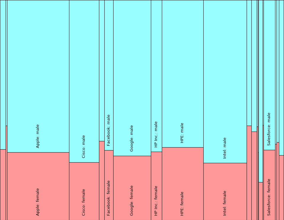
While this data is moderately interesting as a spreadsheet, it takes some careful study to get a sense of the diversity at a particular company. Rather than using a spreadsheet, the summary data can be represented hierarchically as a tree, which provides additional insight. For example, below we show the number of employees who identify as male and female at each of the 22 companies in the dataset. This is just a sub-part of the data (summing over all races and all job categories). Each node contains the count of employees summed across its children nodes. For example, the root node contains 354964 employees, which is the sum of the number of employees at the 22 different companies. 23andMe has 297 employees, 148 of whom identify as male and 149 of whom identify as female.
354964
│
├──23andMe: 297
│  │
│  ├──male: 148
│  │
│  └──female: 149
│
├──Adobe: 7162
│  │
│  ├──male: 4859
│  │
│  └──female: 2303
│
├──Airbnb: 1917
│  │
│  ├──male: 1095
│  │
│  └──female: 822
│
├──Apple: 77192
│  │
│  ├──male: 53456
│  │
│  └──female: 23736
│
├──Cisco: 37526
│  │
│  ├──male: 27681
│  │
│  └──female: 9845
│
├──eBay: 6611
│  │
│  ├──male: 4238
│  │
│  └──female: 2373
│
├──Facebook: 11241
│  │
│  ├──male: 7676
│  │
│  └──female: 3565
│
├──Google: 46760
│  │
│  ├──male: 33120
│  │
│  └──female: 13640
│
├──HP Inc.: 13613
│  │
│  ├──male: 9393
│  │
│  └──female: 4220
│
├──HPE: 51989
│  │
│  ├──male: 34794
│  │
│  └──female: 17195
│
├──Intel: 54135
│  │
│  ├──male: 40084
│  │
│  └──female: 14051
│
├──Intuit: 5911
│  │
│  ├──male: 3373
│  │
│  └──female: 2538
│
├──LinkedIn: 6655
│  │
│  ├──male: 3978
│  │
│  └──female: 2677
│
├──Lyft: 1433
│  │
│  ├──male: 824
│  │
│  └──female: 609
│
├──MobileIron: 506
│  │
│  ├──male: 350
│  │
│  └──female: 156
│
├──Nvidia: 5348
│  │
│  ├──male: 4429
│  │
│  └──female: 919
│
├──Pinterest: 944
│  │
│  ├──male: 537
│  │
│  └──female: 407
│
├──Salesforce: 14716
│  │
│  ├──male: 10019
│  │
│  └──female: 4697
│
├──Square: 1711
│  │
│  ├──male: 1119
│  │
│  └──female: 592
│
├──Twitter: 2952
│  │
│  ├──male: 1908
│  │
│  └──female: 1044
│
├──Uber: 5885
│  │
│  ├──male: 4149
│  │
│  └──female: 1736
│
└──View: 460
   │
   ├──male: 382
   │
   └──female: 78
Note that we added a root node with no label to tie the categories together into a single tree.
While this tree representation helps us to make comparisons, once we add in the other factors (job title and race), the data will be sliced in such a way that we will lack an intuitive sense of the relative diversity at the different companies. It would be much better to see a visual representation of the data, which is the role information visualization plays in computing and in data science.
How can we visualize this information in an effective way? We can use Treemaps, which are an excellent tool for visualizing hierarchical data. Here, for example, is a treemap of gender diversity across the 22 companies:
Treemap of gender diversity across companies
Looking at the data in this form, we can immediately see the proportion of males and females at each company, as well as how different Silicon Valley tech companies compare to each other in terms of gender diversity. The treemap also visualizes the relative size of the workforce at each company, showing that comparatively gender-balanced companies tend to have too small a workforce to even give them a legible label in the treemap.
In general, treemaps are a space-constrained method for visualizing hierarchical structures that present a sense of “mass” and proportionality in a way that the typical tree diagram shown above does not. Treemaps allow the viewer to compare leaves and sub-trees even at varying depths in the tree, and to spot patterns and exceptions. Ben Shneiderman designed treemaps during the 1990s as a way to visualize the contents of a file system. This technique has since been used to visualize many different types of data, including stock portfolios, oil production, a gene ontology, stimulus spending, and more. The original idea has been extended in many interesting ways.
In this assignment, you will write code to draw treemaps to visualize this diversity data from Silicon Valley tech companies in a number of ways.
Silicon Valley EEO-1 Data
We have reformatted the data collected by
Reveal
slightly and included it as
Reveal_EEO1_for_2016.csv in the data directory of this programming
assignment. Each row of the dataset contains the following:
company: Company nameyear: Currently2016onlyrace: Possible values:American_Indian_Alaskan_Native,Asian,Black_or_African_American,Latino,Native_Hawaiian_or_Pacific_Islander,Two_or_more_races,Whitegender: Possible values:male,female(Non-binary gender is not included in EEO-1 reports)job_category: Possible values:Administrative support,Craft workers,Executive/Senior officials & Mgrs,First/Mid officials & Mgrs,laborers and helpers,operatives,Professionals,Sales workers,Service workers,Technicianscount: For the job category, company, race, and gender specified by that row, an integer representing the number of employees (as of 2016) in that job category at that company who identify with that race and gender
Note that this data is in CSV format. As an example, the row
"Adobe",2016,"Latino","male","Professionals",75 indicates that in 2016,
Adobe had 75 employees in the job category Professionals who identified
as Latino and male. Because the data includes 22 companies, the csv file
contains a header row plus 3080 data rows (22 companies * 2 gender categories *
7 race categories * 10 job categories). In total, this CSV file contains
data about 354,964 employees at those 22 companies.
TASK 0
Your warm-up task is to complete the following function in diversity.py:
def load_diversity_data(filename):
In this function, we already read in the data from the CSV file and store it in a pandas dataframe. Modify this function so that, before returning this DataFrame, the function prints out the following basic summary statistics to give a high-level view of the data:
- List how many companies are included in the data, in addition to the names of the companies. Do not include any counts of employees for the companies
- Explain how many employees in total are included in the data
- Summarize how many employees of each gender are included in the dataset
- Summarize how many employees of each race are included in the dataset
- Summarize how many employees of each job_category are included in the dataset
Your code should generalize. For example, it should calculate the number of companies from the dataframe, rather than using a hard-coded value of 22. You should compute these summary statistics primarily using the pandas Python package. An example output follows. Your output does not have to match this format exactly, but it should include the same information and be aesthetically pleasing.
Diversity data comes from the following 22 companies:
23andMe, Adobe, Airbnb, Apple, Cisco, eBay, Facebook,
Google, HP Inc., HPE, Intel, Intuit, LinkedIn, Lyft,
MobileIron, Nvidia, Pinterest, Salesforce, Square, Twitter,
Uber, View

The data includes 354964 employees

#############
gender
#############
  female :  107352
  male :  247612

#############
race
#############
  American_Indian_Alaskan_Native :  1165
  Asian :  96171
  Black_or_African_American :  17832
  Latino :  25767
  Native_Hawaiian_or_Pacific_Islander :  1146
  Two_or_more_races :  5871
  White :  207012

#############
job_category
#############
  Administrative support :  18792
  Craft workers :  543
  Executive/Senior officials & Mgrs :  3536
  First/Mid officials & Mgrs :  52036
  Professionals :  204025
  Sales workers :  42615
  Service workers :  904
  Technicians :  32057
  laborers and helpers :  190
  operatives :  266
Testing Task 0
To do small scale testing of Task 0, fire up ipython3 in your
pa7 directory and then run the following commands:
In [1]: run diversity.py
In [2]: data = load_diversity_data("data/Reveal_EEO1_for_2016.csv")
If Task 0 is correctly implemented, it should produce output similar to the output above. To reiterate, it is not necessary to match this formatting precisely.
Representing tree nodes
While storing this data in a dataframe lets us start examining the data, drawing a treemap will be much easier if we represent the data as a tree. We will construct the tree such that each level of the tree represents a particular employee characteristic. For instance, one level of the tree might represent job categories, while another level of the tree might represent gender.
We provide a class, TreeNode in the file treenode.py,
that you can use to represent tree data. The
class is useful for representing the diversity data, but it is not
specific to the diversity data.
Take into account that this is not the same Tree class we saw in class.
However, its internal representation is similar: a TreeNode object
represents a node on a tree, each node has a few attributes,
and the node’s children are stored in a list. The public interface for this
class includes:
- a constructor for creating a tree node,
- properties for a
countattribute (integer), alabelattribute (string), and averbose_labelattribute (string). - setters for these attributes
- a list of children nodes
- a method,
num_children, that returns the number of children the node has - a method,
tree_print, for printing the tree rooted at that node for debugging purposes
We can use this class to represent our employee diversity data by using the
count attribute to hold the number of employees and the label attribute
to hold the name of the category that node represents. For instance, in the
gender level of the tree, a label would be either female or male.
Note that, for all levels other than the first non-root level of the tree,
multiple nodes on that level can (and should) have the same label.
We will use the attribute verbose_label to store a string representation
of the full path to a node, which we will use to print the full path when
displaying the treemap. We elaborate on this requirement in Task 1.
If you are wondering why we are using generic names—label and count— rather than diversity category or number of employees, it is because this approach allows your treemap implementation to generalize to situations beyond employment diversity data.
We provide the following function, data_to_tree, that creates a tree
from a pandas DataFrame following a specified hierarchy. Note that it does
so by calling a helper function, create_st, which recursively creates
sub-trees.
def data_to_tree(data, hierarchy):
    '''
    Converts a pandas DataFrame to a tree (using TreeNode)
    following a specified hierarchy

    Inputs:
      data: (pandas.DataFrame) the data to be represented
            as a tree
      hierarchy: (list of strings) a list of column names
                 to be used as the levels of the tree in the
                 order given. Note that all strings in the
                 hierarchy must correspond to column names
                 in data

    Returns: a tree (using the TreeNode class) representation of
             data
    '''
A sample call of data_to_tree follows:
In [1]: run diversity.py
In [2]: data = load_diversity_data("data/Reveal_EEO1_for_2016.csv")
In [3]: example_tree = data_to_tree(data, ["company", "gender"])
In [4]: example_tree.tree_print()
This builds a tree similar to the company-by-company breakdown of employees’
genders shown in the introduction. The tree returned, however, lacks counts
for the internal (non-leaf) nodes, which in this particular case is just the
root node. You will fill in these counts in Task 1.
Replacing line 3 with
example_tree = data_to_tree(data, ["company", "job_category", "race", "gender"])
builds a tree on all four categories. For this deeper tree, the missing counts
for internal nodes will be more obvious.
As shown above, after building a tree using the data_to_tree function,
you can use the tree_print method of the TreeNode class to print the tree for
debugging purposes.
TASK 1
Note that the tree we return from data_to_tree contains a meaningful
count attribute (as opposed to None) only for leaf nodes. Furthermore,
the verbose_label attribute is None for all nodes. In Task 1, you will
complete the following two recursive functions in treemap.py to
respectively compute count for all internal nodes and to set the
verbose_label for all nodes other than the root of the tree.
Your solution to each must be recursive. Non-recursive solutions (i.e.,
functions that do not call themselves with an input that is in some way
smaller) will not receive credit for this task. Furthermore, each
function should be generalizable, working for a tree of any depth.
Note that each of these functions requires fewer than ten lines of code.
def compute_internal_counts(t):
    '''
    Assign a count to the interior nodes.  The count of the leaves
    should already be set.  The count of an internal node is the sum
    of the counts of its children.

    Inputs:
        t: a tree

    Returns:
        The count at that node. This is count for leaf nodes, and the sum of
            the counts of the children of internal nodes. The input tree t
            should be destructively modified so that every internal node's
            count is set to be the sum of the counts of its children.
    '''
def compute_verbose_labels(t, prefix=None):
    '''
    Assign a verbose label to non-root nodes. Verbose labels contain the
    full path to that node through the tree. For example, following the
    path "Google" --> "female" --> "white" should create the verbose label
    "Google: female: white"

    Inputs:
        t: a tree

    Outputs:
        No explicit output. The input tree t should be modified to contain
            verbose labels for all non-root nodes
    '''
Testing Task 1
Please test your code incrementally as you write it, developing appropriate test cases on your own. Unlike for other programming assignments, we do not provide you with test cases.
To do small scale testing of compute_internal_counts(t),
fire up ipython3 and then run the following commands:
In [1]: run diversity.py
In [2]: data = load_diversity_data("data/Reveal_EEO1_for_2016.csv")
In [3]: example_tree = data_to_tree(data, ["company", "gender"])
In [4]: run treemap.py
In [5]: compute_internal_counts(example_tree)
In [6]: example_tree.tree_print()
If you have implemented compute_internal_counts correctly, the tree
this builds and prints will show the same company-by-company breakdown of
employees’ genders shown in the introduction. Like the output shown
in the introduction, this tree will now show the count for all nodes, not
just the leaf nodes.
It is up to you to decide how you would like to test
compute_verbose_labels.
Recall that the tree_print method is help for examining the state of the
tree while debugging, but does not show the verbose_label. That said,
you are welcome to modify it for your own testing purposes (e.g.,
to perhaps test your compute_verbose_labels implementation). Do not
submit your modified version of tree_print.
Drawing Treemaps
The treemap algorithm takes a weighted tree and an initial bounding rectangle as arguments. In a weighted tree, the weight of a leaf is an application-specific cost and the weight of a subtree is the sum of the weights of its children. The treemap algorithm assigns regions in the rectangle to the leaves of the tree. The size of the region assigned to a leaf (itself a rectangle) is a function of the leaf’s relative weight and its placement is a function of its position in the tree.
Here are two examples that we will use to make this concept more concrete. Example Tree 1 shows a tree that breaks the data down only by job category:
: 354964
│
├──Administrative support: 18792
│
├──Craft workers: 543
│
├──Executive/Senior officials & Mgrs: 3536
│
├──First/Mid officials & Mgrs: 52036
│
├──laborers and helpers: 190
│
├──operatives: 266
│
├──Professionals: 204025
│
├──Sales workers: 42615
│
├──Service workers: 904
│
└──Technicians: 32057
We created this first tree in ipython3 with the following calls:
In [1]: run diversity.py
In [2]: data = load_diversity_data("data/Reveal_EEO1_for_2016.csv")
In [3]: example_tree = data_to_tree(data, ["job_category"])
In [4]: run treemap.py
In [5]: compute_internal_counts(example_tree)
In [6]: example_tree.tree_print()
Note that the sample code will only show the count for the root node if
you correctly implemented your compute_internal_counts function.
This tree represents the breakdown by job category summing across
all companies and genders and races.
Example Tree 2 instead shows a tree that first breaks the data down by job category, and then by gender.
: 354964
│
├──Administrative support: 18792
│  │
│  ├──male: 7038
│  │
│  └──female: 11754
│
├──Craft workers: 543
│  │
│  ├──male: 511
│  │
│  └──female: 32
│
├──Executive/Senior officials & Mgrs: 3536
│  │
│  ├──male: 2738
│  │
│  └──female: 798
│
├──First/Mid officials & Mgrs: 52036
│  │
│  ├──male: 36366
│  │
│  └──female: 15670
│
├──laborers and helpers: 190
│  │
│  ├──male: 90
│  │
│  └──female: 100
│
├──operatives: 266
│  │
│  ├──male: 221
│  │
│  └──female: 45
│
├──Professionals: 204025
│  │
│  ├──male: 146371
│  │
│  └──female: 57654
│
├──Sales workers: 42615
│  │
│  ├──male: 29209
│  │
│  └──female: 13406
│
├──Service workers: 904
│  │
│  ├──male: 585
│  │
│  └──female: 319
│
└──Technicians: 32057
   │
   ├──male: 24483
   │
   └──female: 7574
This tree represents the gender breakdown by job category summing across all companies and races. We created it in ipython3 as follows:
In [1]: run diversity.py
In [2]: data = load_diversity_data("data/Reveal_EEO1_for_2016.csv")
In [3]: example_tree = data_to_tree(data, ["job_category", "gender"])
In [4]: run treemap.py
In [5]: compute_internal_counts(example_tree)
In [6]: example_tree.tree_print()
To explain how the treemap algorithm works, we need to describe how to:
- compute the weights
- represent rectangles
- partition the initial bounding rectangle
- use the drawing package
- choose the colors and labels for the rectangles in the resulting partition
Weighting Function:
We use the term weight to refer to the relative proportion of an object
of interest (in this case, the number of employees) represented by a
particular node in the tree.
The weights of the leaves are set at the time the tree is constructed
and can be accessed using the count property. In Task 1, you finished
the function compute_internal_counts, which let you compute count
(the weight) for the internal nodes.
Representing rectangles
A rectangle can be represented using points on two opposing corners (upper left and lower right corners, for example) or a single point (the origin) and a width and a height. We use the latter representation for our implementation and in this description, but either works. In most of our examples below, we use a bounding rectangle that has an origin of (0, 0), a height of 1.0, and a width of 1.0. (Note: these values are naturally unit-less.)
It will be helpful when you try to interpret the diagrams below to know that the origin (0,0) for our coordinate system is in the upper left corner, rather than lower left corner, which might seem more natural. We made this choice because this coordinate system matches the coordinate system of many drawing packages, including ours.
Partitioning the initial bounding rectangle
Once the tree is decorated with the correct weights (counts),
we need to divide
an initial bounding rectangle into a collection of smaller rectangles
based on the shape of the tree and the distribution of the weights
(“mass”). Each rectangle in the resulting partition will have an
associated label: the verbose_label for that node.
To describe how regions of the bounding rectangle are allocated in the treemap algorithm, we will start by looking at the treemap from Example Tree 1, above.
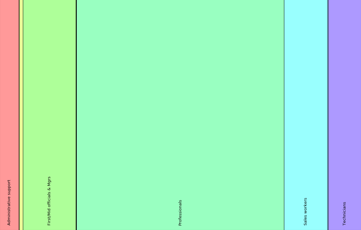
Treemap splitting by job category
The treemap algorithm splits the initial rectangle into sub-rectangles—one per child of the root. The proportion of a child’s sub-rectangle is determined by its weight as a fraction of the total weight of its parent. For example, the treemap algorithm splits the initial rectangle from left to right into ten pieces, with each piece representing a job category. Note that pieces representing job categories with few employees are too skinny to see clearly in the treemap. Given an initial bounding rectangle with its origin at (0,0), a width of 1.0 and a height of 1.0, the resulting partition would be:
| Verbose Label | X | Y | Width | Height |
|---|---|---|---|---|
Administrative support |
0.000 | 0.000 | 0.053 | 1.000 |
Craft workers |
0.053 | 0.000 | 0.002 | 1.000 |
Executive/Senior officials & Mgrs |
0.054 | 0.000 | 0.010 | 1.000 |
First/Mid officials & Mgrs |
0.064 | 0.000 | 0.147 | 1.000 |
laborers and helpers |
0.211 | 0.000 | 0.001 | 1.000 |
operatives |
0.212 | 0.000 | 0.001 | 1.000 |
Professionals |
0.212 | 0.000 | 0.575 | 1.000 |
Sales workers |
0.787 | 0.000 | 0.120 | 1.000 |
Service workers |
0.907 | 0.000 | 0.003 | 1.000 |
Technicians |
0.910 | 0.000 | 0.090 | 1.000 |
Each row corresponds to a rectangle, and each rectangle is associated
with a node in Example Tree 1.
In this case, the children of the tree’s root are all leaf nodes, and that
is what we visualize on the treemap. The first column in this table identifies
the tree nodes’ verbose label (verbose_label), which in this specific
case happens to be identical to label as the tree contains only one
level beyond the root
node. The next four columns contain the components
of the rectangles rounded to three digits for clarity. Notice that 57.5%
of the initial rectangle (by width) went to Professionals, while 1.0% went
to Executive/Senior officials & Mgrs. These correspond to their relative
weights of 204025/354964 and 3536/354964.
While making tables like the one above is not part of this assignment, writing strategic print statements to display analogous data while you are initially writing and debugging your program will help you to isolate errors that are due to your generation of the rectangles, as opposed to errors drawing the rectangles you generate. We highly recommend you print out such information, and we will ask you to show us these sorts of print-outs when helping you to debug your code.
We will now move on to Example Tree 2 (breaking down by job category and then by gender), which introduces additional complexity by having multiple levels of the tree beyond the root.
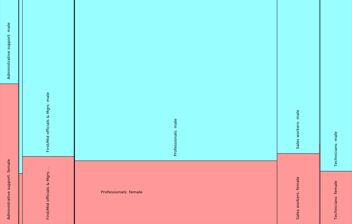
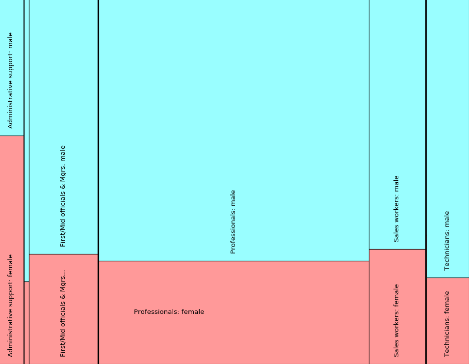
Treemap splitting by job category and gender
The treemap algorithm first splits the initial rectangle left to right by job category, just as for Example Tree 1. There is a second step, however, for Example Tree 2 because it contains another level. This additional level of the tree represents the gender distribution within that job category. Notice that while the proportions for a particular job category are split the same as in the treemap for Example Tree 1, there is a subsequent split within each of those rectangles. That is, the rectangle representing a particular job category is then split by gender.
Pay close attention to the fact that the orientation of the split has also changed after progressing to this next level; rectangles representing gender are split (allocated) from top to bottom, rather than from left to right. As a result, the width for a particular job category for Example Tree 2 is identical to the width for that job category in Example Tree 1. However, whereas the height of all nodes in the first example was 1.000, the height is distributed proportionally by gender in this second example. Assuming the initial bounding rectangle has its origin at (0,0), a width 1.0, and a height 1.0, the resulting partition would be:
| Verbose Label | X | Y | Width | Height |
|---|---|---|---|---|
Administrative support: male |
0.000 | 0.000 | 0.053 | 0.375 |
Administrative support: female |
0.000 | 0.375 | 0.053 | 0.625 |
Craft workers: male |
0.053 | 0.000 | 0.002 | 0.941 |
Craft workers: female |
0.053 | 0.941 | 0.002 | 0.059 |
Executive/Senior officials & Mgrs: male |
0.054 | 0.000 | 0.010 | 0.774 |
Executive/Senior officials & Mgrs: female |
0.054 | 0.774 | 0.010 | 0.226 |
First/Mid officials & Mgrs: male |
0.064 | 0.000 | 0.147 | 0.699 |
First/Mid officials & Mgrs: female |
0.064 | 0.699 | 0.147 | 0.301 |
laborers and helpers: male |
0.211 | 0.000 | 0.001 | 0.474 |
laborers and helpers: female |
0.211 | 0.474 | 0.001 | 0.526 |
operatives: male |
0.212 | 0.000 | 0.001 | 0.831 |
operatives: female |
0.212 | 0.831 | 0.001 | 0.169 |
Professionals: male |
0.212 | 0.000 | 0.575 | 0.717 |
Professionals: female |
0.212 | 0.717 | 0.575 | 0.283 |
Sales workers: male |
0.787 | 0.000 | 0.120 | 0.685 |
Sales workers: female |
0.787 | 0.685 | 0.120 | 0.315 |
Service workers: male |
0.907 | 0.000 | 0.003 | 0.647 |
Service workers: female |
0.907 | 0.647 | 0.003 | 0.353 |
Technicians: male |
0.910 | 0.000 | 0.090 | 0.764 |
Technicians: female |
0.910 | 0.764 | 0.090 | 0.236 |
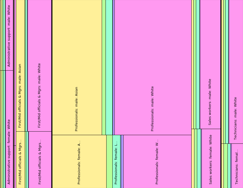
While Example Tree 2 has two levels, your code should be able to construct treemaps from trees with an arbitrarily large number of levels. The orientation of the partitions alternates between left-to-right and top-to-bottom as we move down each level of the tree. If our tree had a third level beyond these two, that third level would again have been split left-to-right. Alternating the split at each level in the tree produces a picture that is much easier to understand than one in which all the partitions have the same orientation. The following treemap visualizes a tree with three levels:
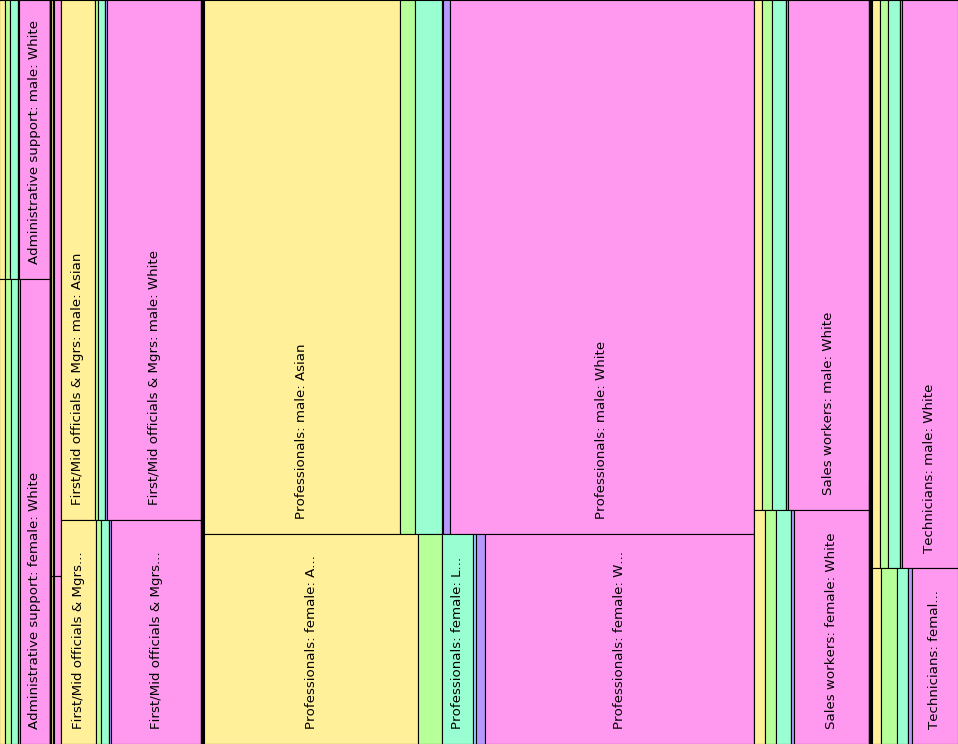
Treemap splitting by job category, gender, and race
Note that the rectangles representing job category (the first level of the tree beyond the root) are split left-to-right. The rectangles representing gender (the second level) are split top-to-bottom. Finally, the rectangles representing race (the final level of the tree) are again split left-to-right.
Using the drawing package
We will be using the ChiCanvas class for drawing rectangles and
text. This class provides a way to create a canvas, draw the outline
of a rectangle, draw a rectangle filled with a particular color, draw
text horizontally and vertically, show a drawing, etc. See the
API for details, including the arguments expected
by the constructor. Note that we have defined X_SCALE_FACTOR and
Y_SCALE_FACTOR in treemap.py, and you should use these as inputs
to the ChiCanvas constructor as specified in the API.
The file sample.py contains a
set of simple examples that use this class.
Our code handles the construction of a canvas for you. The coordinate system for the canvas is the unit square with an origin of (0.0, 0.0) (upper left corner), a width of 1.0, and a height of 1.0. Again, these values are unit-less.
We strongly encourage you to look carefully at the ChiCanvas API
and at sample.py before you get started with drawing.
The ColorKey class allows you to create a key that maps labels to
colors (API). The constructor takes a set of
labels as strings and assigns a color to each label. Given a ColorKey
named ck, you extract the color for a particular label, c, with
the get_color method. For example:
ck.get_color(c)
This class also has a method for drawing a key that shows the mapping
of colors to labels, but we will not use it for this assignment. We have
again provided a sample file (sample_ck.py) demonstrating how to
create a color key. We encourage you to look carefully at the ColorKey
API and at sample_ck.py before you get started with drawing.
Choosing labels and colors
Each rectangle in the partition that results from the previous step is
associated with a leaf node in our tree. Because, for all levels other
than the first, multiple leaf nodes will share the same label,
we use verbose_label as the text we display. This verbose label, generated
using one of the functions you wrote in Task 1, specifies the full path
to that node in the tree.
Although you will want to use the verbose_label for the text itself,
it makes sense to visualize leaf nodes that represent the same category
as the same color in order to provide the viewer quick intuition about how the
data is distributed. That is, if job category and gender are both levels of
the tree (as in Example Tree 2), yet gender is the deepest
level of the tree (furthest from the root node), all rectangles representing
employees of a particular gender should be the same color. For example,
Professionals: female and Technicians: female (as with females of all
job categories) should be drawn using the same color.
You will construct a color key using the labels from the nodes in your partition and then use this key and the labels to determine the appropriate colors when you draw the partition rectangles. (Hint: we found the Python set data structure useful when compiling the labels for the color key.) Furthermore, we recommend that you think about whether you already have an attribute for the nodes of your tree that can be used to determine which nodes should be visualized with the same color.
You should orient the labels in the rectangles horizontally or
vertically depending on whether the width or the height of the
rectangle is larger. If the width and the height are the same, orient
the labels horizontally. Do not draw the label for any rectangle that
has a height or width of less than .03. (We have defined a constant,
MIN_RECT_SIDE_FOR_TEXT for this purpose.) Note that labels that
are too long will be clipped to fit automatically by the drawing
package.
TASK 2
Your second (and most complicated) task is to complete the function:
def draw_treemap(t,
                 bounding_rec_height=1.0,
                 bounding_rec_width=1.0,
                 output_filename=None)
in treemap.py, which takes a tree, optionally
the height and width of the initial
bounding rectangle, and an optional filename, constructing a canvas
and then drawing a treemap for t using the specified initial
rectangle. If the output filename is None, then your code should
“show” the canvas. Otherwise, it should save the canvas in the
specified file.
You may assume that the tree t (an object of class TreeNode)
has label defined for all nodes (leaf or internal) and
count defined for all leaf nodes. As part of your implementation of
draw_treemap, you will likely want to call the functions you wrote in
Task 1 to compute count for internal nodes and set verbose_label
throughout the tree.
As in Task 1, your functions for computing the partition for the treemap must be recursive. Also, you may not make any assumptions about the number of levels in the tree.
You are on your own for deciding what functions to write. We highly
recommend that you figure out what functions you need before you start
writing code and test those functions as you go. Including draw_treemap,
our solution has three functions in addition to the two from Task 1. Our
solution is roughly 50 lines of code.
Testing Task 2
We created the treemap you saw above (splitting by job category, gender, and race) by running the following commands:
In [1]: run diversity.py
In [2]: data = load_diversity_data("data/Reveal_EEO1_for_2016.csv")
In [3]: example_tree = data_to_tree(data, ["job_category", "gender", "race"])
In [4]: run treemap.py
In [5]: compute_internal_counts(example_tree)
In [6]: compute_verbose_labels(example_tree)
In [7]: draw_treemap(example_tree)
TASK 3
Rather than always creating a treemap of the full set of data, you might first want to subset the data. For example, rather than trying to look at a particular small area of interest to you in a larger treemap, you could prune the tree, which involves removing nodes (and their children) that have a particular characteristic.
In this task, you will write a function that takes as input a tree, as well
as a list of labels identifying nodes to discard (values_to_discard).
Your function must recursively traverse the tree, returning a copy of this
original tree with all nodes whose labels are in values_to_discard
removed, along with their children. Do not modify the original tree.
You may assume (without needing to verify) that values_to_discard does
not contain all labels for a particular level. If it did contain all labels
for a particular level (e.g., it included both male and female),
no employees would be left in the tree, and the tree’s structure would also
be broken. Do not worry about that case.
Because the counts for internal nodes will change if part of the tree is
pruned, the copy of the tree your function returns should contain count
for all leaf nodes, but set count to None for all internal nodes.
You may assume that the original_sub_tree passed to the function has
correct counts for all nodes (leaf nodes and internal nodes) in the tree.
In particular, you will complete the following function:
def prune_tree(original_sub_tree, values_to_discard):
  '''
  Returns a tree with any node whose label is in the list values_to_discard
  (and thus all of its children) pruned. This function should return a copy
  of the original tree and should not destructively modify the original tree.
  The pruning step must be recursive.

  Inputs:
      original_sub_tree: (TreeNode) a tree of type TreeNode whose internal
                counts have been computed. That is, compute_internal_counts()
                must have been run on this tree.
      values_to_discard: (list of strings) A list of strings specifying the
                labels of nodes to discard

  Returns: a new TreeNode representing the pruned tree
  '''
Keep in mind that this task (like others in this assignment)
is conceptually complex, yet does not require much code.
Our prune_tree implementation contains fewer than 10 lines of code.
Testing Task 3
For example, to create a tree containing the full set of data, and then to
prune the tree to remove all data from employees in the job categories Technicians
and Sales workers, as well as all data from employees who identify as
Two_or_more_races or as male, one could make the following series of calls
(after you
complete your prune_tree function):
In [1]: run diversity.py
In [2]: data = load_diversity_data("data/Reveal_EEO1_for_2016.csv")
In [3]: example_tree = data_to_tree(data, ["job_category", "race", "gender"])
In [4]: run treemap.py
In [5]: compute_internal_counts(example_tree)
In [6]: pruned_tree = prune_tree(example_tree, ["Technicians", "Sales workers", "Two_or_more_races", "male"])
In [7]: compute_internal_counts(pruned_tree)
In [8]: pruned_tree.tree_print()
Line 8 should produce the following output if your functions from Task 1 and Task 3 are implemented correctly:
: 84812
│
├──Administrative support: 11416
│  │
│  ├──American_Indian_Alaskan_Native: 78
│  │  │
│  │  └──female: 78
│  │
│  ├──Asian: 1363
│  │  │
│  │  └──female: 1363
│  │
│  ├──Black_or_African_American: 1349
│  │  │
│  │  └──female: 1349
│  │
│  ├──Latino: 1614
│  │  │
│  │  └──female: 1614
│  │
│  ├──Native_Hawaiian_or_Pacific_Islander: 62
│  │  │
│  │  └──female: 62
│  │
│  └──White: 6950
│     │
│     └──female: 6950
│
├──Craft workers: 32
│  │
│  ├──American_Indian_Alaskan_Native: 1
│  │  │
│  │  └──female: 1
│  │
│  ├──Asian: 5
│  │  │
│  │  └──female: 5
│  │
│  ├──Black_or_African_American: 0
│  │  │
│  │  └──female: 0
│  │
│  ├──Latino: 4
│  │  │
│  │  └──female: 4
│  │
│  ├──Native_Hawaiian_or_Pacific_Islander: 0
│  │  │
│  │  └──female: 0
│  │
│  └──White: 22
│     │
│     └──female: 22
│
├──Executive/Senior officials & Mgrs: 786
│  │
│  ├──American_Indian_Alaskan_Native: 1
│  │  │
│  │  └──female: 1
│  │
│  ├──Asian: 157
│  │  │
│  │  └──female: 157
│  │
│  ├──Black_or_African_American: 19
│  │  │
│  │  └──female: 19
│  │
│  ├──Latino: 31
│  │  │
│  │  └──female: 31
│  │
│  ├──Native_Hawaiian_or_Pacific_Islander: 0
│  │  │
│  │  └──female: 0
│  │
│  └──White: 578
│     │
│     └──female: 578
│
├──First/Mid officials & Mgrs: 15424
│  │
│  ├──American_Indian_Alaskan_Native: 39
│  │  │
│  │  └──female: 39
│  │
│  ├──Asian: 3871
│  │  │
│  │  └──female: 3871
│  │
│  ├──Black_or_African_American: 550
│  │  │
│  │  └──female: 550
│  │
│  ├──Latino: 864
│  │  │
│  │  └──female: 864
│  │
│  ├──Native_Hawaiian_or_Pacific_Islander: 54
│  │  │
│  │  └──female: 54
│  │
│  └──White: 10046
│     │
│     └──female: 10046
│
├──laborers and helpers: 100
│  │
│  ├──American_Indian_Alaskan_Native: 0
│  │  │
│  │  └──female: 0
│  │
│  ├──Asian: 20
│  │  │
│  │  └──female: 20
│  │
│  ├──Black_or_African_American: 20
│  │  │
│  │  └──female: 20
│  │
│  ├──Latino: 38
│  │  │
│  │  └──female: 38
│  │
│  ├──Native_Hawaiian_or_Pacific_Islander: 0
│  │  │
│  │  └──female: 0
│  │
│  └──White: 22
│     │
│     └──female: 22
│
├──operatives: 45
│  │
│  ├──American_Indian_Alaskan_Native: 0
│  │  │
│  │  └──female: 0
│  │
│  ├──Asian: 3
│  │  │
│  │  └──female: 3
│  │
│  ├──Black_or_African_American: 11
│  │  │
│  │  └──female: 11
│  │
│  ├──Latino: 9
│  │  │
│  │  └──female: 9
│  │
│  ├──Native_Hawaiian_or_Pacific_Islander: 0
│  │  │
│  │  └──female: 0
│  │
│  └──White: 22
│     │
│     └──female: 22
│
├──Professionals: 56697
│  │
│  ├──American_Indian_Alaskan_Native: 165
│  │  │
│  │  └──female: 165
│  │
│  ├──Asian: 22410
│  │  │
│  │  └──female: 22410
│  │
│  ├──Black_or_African_American: 2449
│  │  │
│  │  └──female: 2449
│  │
│  ├──Latino: 3226
│  │  │
│  │  └──female: 3226
│  │
│  ├──Native_Hawaiian_or_Pacific_Islander: 302
│  │  │
│  │  └──female: 302
│  │
│  └──White: 28145
│     │
│     └──female: 28145
│
└──Service workers: 312
   │
   ├──American_Indian_Alaskan_Native: 2
   │  │
   │  └──female: 2
   │
   ├──Asian: 46
   │  │
   │  └──female: 46
   │
   ├──Black_or_African_American: 17
   │  │
   │  └──female: 17
   │
   ├──Latino: 137
   │  │
   │  └──female: 137
   │
   ├──Native_Hawaiian_or_Pacific_Islander: 6
   │  │
   │  └──female: 6
   │
   └──White: 104
      │
      └──female: 104
Final Testing
For when you have completed most (or all) of the tasks, we have written a main function that lets you test your functionality. Note that calling
python3 diversity.py -i data/Reveal_EEO1_for_2016.csv
from the command line, not ipython3, generates the following series of five treemaps. It only shows one at a time; to close a treemap and move on to the next, either click the x in the corner or hit Ctrl-W on your keyboard.
Treemap of gender diversity by job category
Treemap of gender and racial diversity by job category
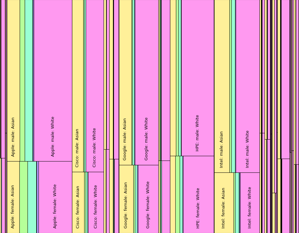
Treemap of gender and racial diversity by company
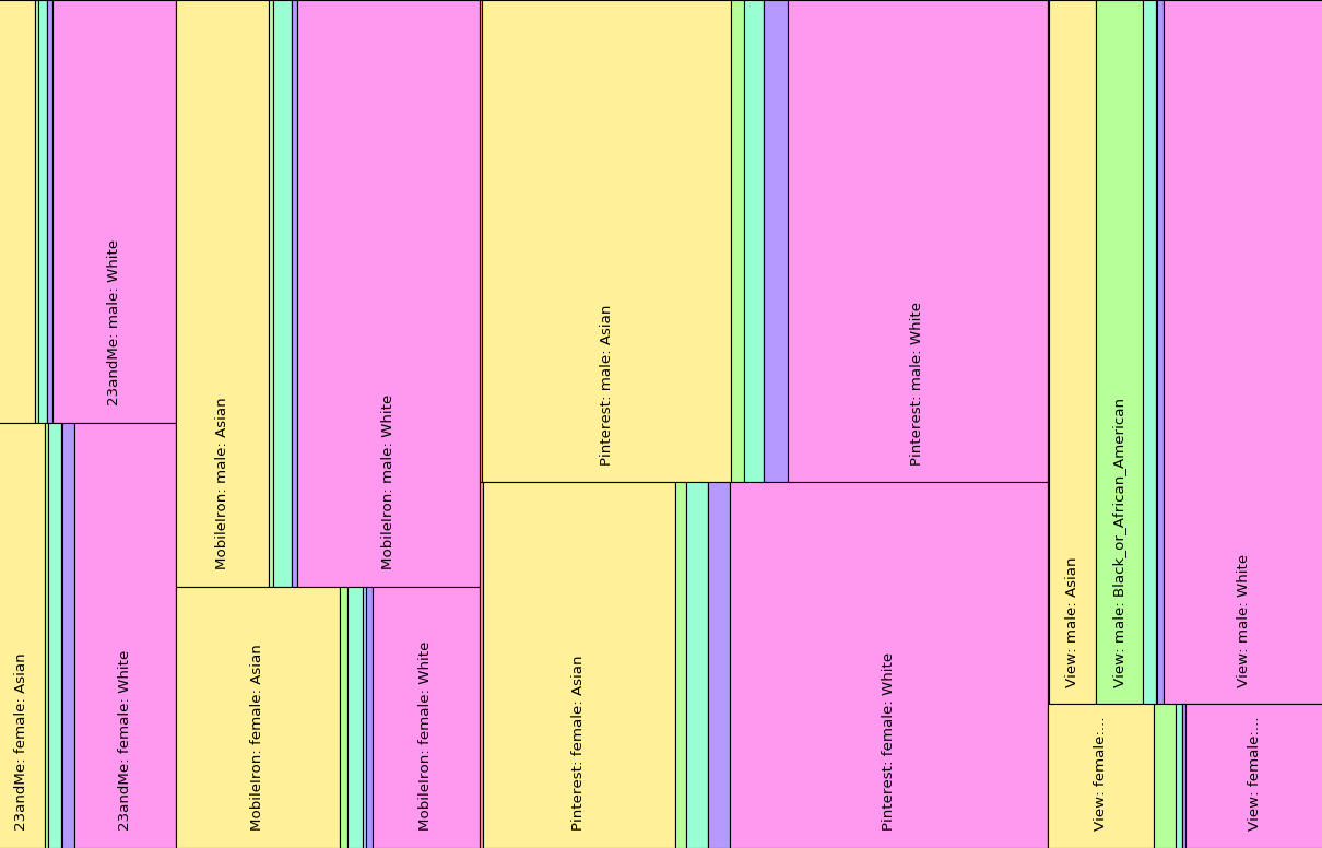
Gender and racial diversity of companies with fewer than 1,000 employees
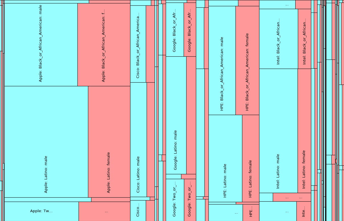
A view of the non-white and non-asian Silicon Valley workforce
Getting started
We have seeded your repository with a directory for this assignment.
To pick it up, change to your cmsc12100-aut-17-username directory
(where the string username should be replaced with your username)
and then run the command: git pull upstream master. You should
also run git pull to make sure your local copy of your repository
is in sync with the server.
See pa7/README.txt for a description of the contents of this
directory.
Submission
To submit your assignment, make sure that you have:
- put your name at the top of your file,
- registered for the assignment using chisubmit,
- added, committed, and pushed your code to the git server, and
- run the chisubmit submission command.
chisubmit student assignment register pa7

git add diversity.py
git add treemap.py

git commit -m "final version ready for submission"
git push

chisubmit student assignment submit pa7
Remember to push your code to the server early and often!
Acknowledgments: Gordon Kindlmann originally recommended drawing treemaps as good topic for an assignment.